New post test

Posted on March 18, 2017

An initial example using knitpost R script, see post by JFisher, for quickly converting R-markdown (*.rmd) into markdown (*.md) with the associated images and such…

based on KnitPost

see http://jfisher-usgs.github.io/r/2012/07/03/knitr-jekyll/

The knitr package provides an easy way to embed R code in a Jekyll-Bootstrap blog post. The only required input is an R Markdown source file. The name of the source file used to generate this post is 2012-07-03-knitr-jekyll.Rmd, available here. Steps taken to build this post are as follows:

Step 1

Create a Jekyll-Boostrap blog if you don’t already have one. A brief tutorial on building this blog is available here.

Step 2

Open the R Console and process the source file:

KnitPost <- function(input, base.url = "/") {
  require(knitr)
  opts_knit$set(base.url = base.url)
  fig.path <- paste0("figs/", sub(".Rmd$", "", basename(input)), "/")
  opts_chunk$set(fig.path = fig.path)
  opts_chunk$set(fig.cap = "center")
  render_jekyll()
  knit(input, envir = parent.frame())
}
KnitPost("2012-07-03-knitr-jekyll.Rmd")

Step 3

Move the resulting image folder 2012-07-03-knitr-jekyll and Markdown file 2012-07-03-knitr-jekyll.md to the local jfisher-usgs.github.com git repository. The KnitPost function assumes that the image folder will be placed in a figs folder located at the root of the repository.

Step 4

Add the following CSS code to the /assets/themes/twitter-2.0/css/bootstrap.min.css file to center images:

[alt=center] {
  display: block;
  margin: auto;
}

Thats it.

Here are a few examples of embedding R code:

summary(cars)

##      speed           dist       
##  Min.   : 4.0   Min.   :  2.00  
##  1st Qu.:12.0   1st Qu.: 26.00  
##  Median :15.0   Median : 36.00  
##  Mean   :15.4   Mean   : 42.98  
##  3rd Qu.:19.0   3rd Qu.: 56.00  
##  Max.   :25.0   Max.   :120.00

par(mar = c(4, 4, 0.1, 0.1), omi = c(0, 0, 0, 0))
plot(cars)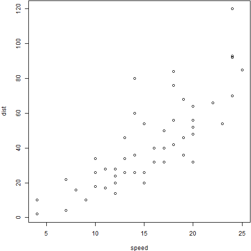

Figure 1-1: Caption

par(mar = c(2.5, 2.5, 0.5, 0.1), omi = c(0, 0, 0, 0))
filled.contour(volcano)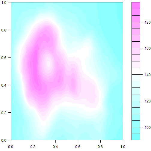

Figure 2-1: Caption

And dont forget your session information for proper reproducible research.

sessionInfo()

## R version 3.3.2 (2016-10-31)
## Platform: x86_64-w64-mingw32/x64 (64-bit)
## Running under: Windows >= 8 x64 (build 9200)
## 
## locale:
## [1] LC_COLLATE=English_United States.1252 
## [2] LC_CTYPE=English_United States.1252   
## [3] LC_MONETARY=English_United States.1252
## [4] LC_NUMERIC=C                          
## [5] LC_TIME=English_United States.1252    
## 
## attached base packages:
## [1] stats     graphics  grDevices utils     datasets  methods   base     
## 
## other attached packages:
## [1] knitr_1.15.1
## 
## loaded via a namespace (and not attached):
## [1] magrittr_1.5  tools_3.3.2   yaml_2.1.14   stringi_1.1.2 highr_0.6    
## [6] stringr_1.1.0 evaluate_0.10

R Markdown

This is an R Markdown document. Markdown is a simple formatting syntax for authoring HTML, PDF, and MS Word documents. For more details on using R Markdown see http://rmarkdown.rstudio.com.

When you click the Knit button a document will be generated that includes both content as well as the output of any embedded R code chunks within the document. You can embed an R code chunk like this:

summary(cars)

##      speed           dist       
##  Min.   : 4.0   Min.   :  2.00  
##  1st Qu.:12.0   1st Qu.: 26.00  
##  Median :15.0   Median : 36.00  
##  Mean   :15.4   Mean   : 42.98  
##  3rd Qu.:19.0   3rd Qu.: 56.00  
##  Max.   :25.0   Max.   :120.00

Including Plots

You can also embed plots, for example:

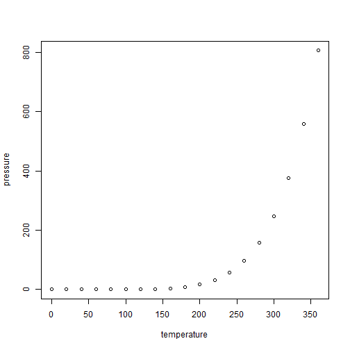
Note that the echo = FALSE parameter was added to the code chunk to prevent printing of the R code that generated the plot.