PRAMS Data Analysis
(Asynchronous-Online)
PRAMS Data
About PRAMS
PRAMS is the Pregnancy Risk Assessment Monitoring System (PRAMS). According to the CDC’s website for About PRAMS:
PRAMS is the Pregnancy Risk Assessment Monitoring System. It is a joint surveillance project between state, territorial, or local health departments and CDC’s Division of Reproductive Health. PRAMS was developed in 1987 to reduce infant morbidity and mortality by influencing maternal behaviors before, during, and immediately after live birth.
The purpose of PRAMS is to find out why some infants are born healthy and others are not. The survey asks new mothers questions about their pregnancy and their new infant. The questions give us important information about the mother and the infant and help us learn more about the impacts of health and behaviors.
Getting the PRAMS Data
- You can request the PRAMS Data from the CDC.
- Once granted access, follow the instructions from the CDC to download the data and sign the data sharing agreement.
- For the purposes of the TIDAL R training session, we will be working with PRAMS Phase 8 ARF (Automated Research File) dataset.
PRAMS Documentation and Resources
- See the details on the PRAMS Questionnaires.
- Learn more about the PRAMS Data Methodology including details on how the samples are weighted.
- Download and Read this helpful paper on PRAMS design and methodology (Shulman, D’Angelo, Harrison, Smith, and Warner, 2018).
- There are also helpful tutorial videos on working with PRAMS data by ASSOCIATION OF STATE AND TERRITORIAL HEALTH OFFICIALS (ASTHO.org).
0. Prework - Before You Begin
Install R Packages
Before you begin, please go ahead and install (or make sure these are already installed) on your computer for these following packages - these are all on CRAN, so you can install them using the RStudio Menu Tools/Install Packages interface:
Create a NEW RStudio Project
BEFORE you being any new analysis project, it is ALWAYS a good idea to begin with the NEW RStudio project.
Go to the RStudio menu “File/New Project” and create your new project (ideally in a NEW directory, but it is also ok to use an exisiting directory/folder on your computer).
This new directory (or folder) will be where all of your files will “live” for your current analysis project.
See the step-by-step instructions for creating a new RStudio project in Module 1.3.2.
1. Get PRAMS Data and Select Subset for Analysis
A. Read-in the PRAMS Phase 8 2016-2021 combined dataset
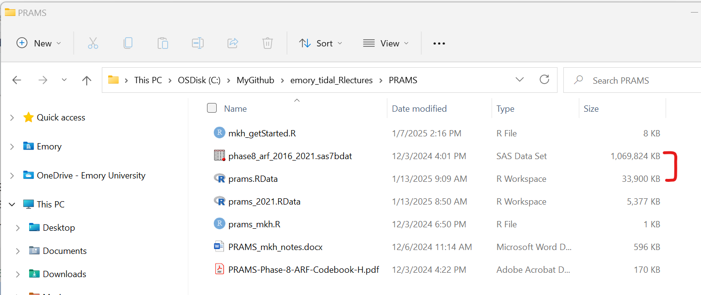
The PRAMS data provided by the CDC will be in SAS format (*.sas7bdat). We can read the native SAS file into R using the haven package and the read_sas() function.
The size of the phase8_arf_2016_2021.sas7bdat dataset is a little over 1GB. So, make sure your computer has enough available memory to fully load this dataset. I will provide some more details below on how we can reduce the size of the dataset and improve the memory issues below.
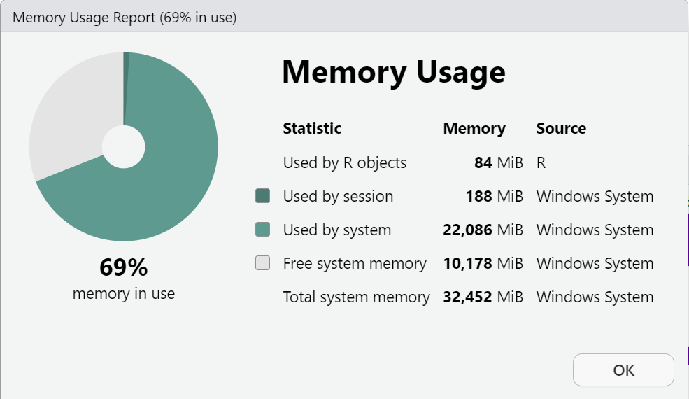
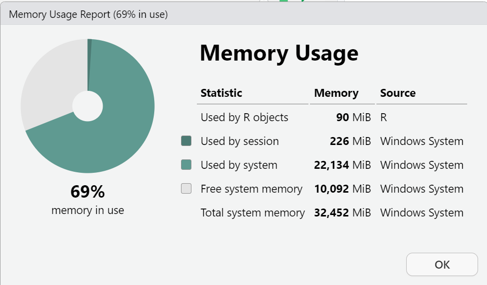
You can check your available memory, by checking your “Global Environment” TAB (upper right window pane) click on the down arrow next to the icon with “XX MiB” just to the left of the little broom:
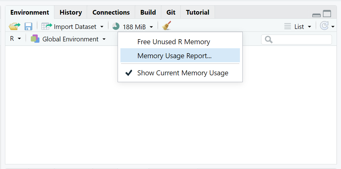
Click on the “Memory Usage Report” to see a detailed breakdown. This window will show:
- Memory used by R objects (in your “Global Environment”)
- Memory used on your computer by your current R Session
- Memory currently in use for everything currently running on your computer (all apps running - active and in background) - you can compare this to your “task manager” memory viewer.
- Free System Memory - when this gets low the “XX MiB” graphic will change color from green - to yellow - to orange - to red. Once you get to red, your R session will most likely crash since there is not enough memory to perfom operations or run analyses.
This is a screen shot of my computer (yours will look different) BEFORE I load the PRAMS dataset.
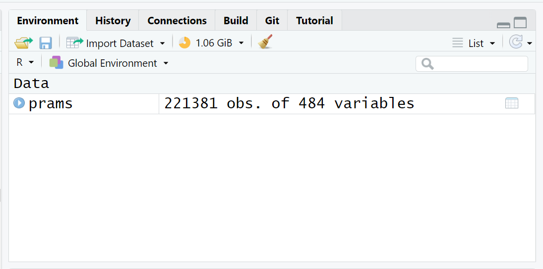
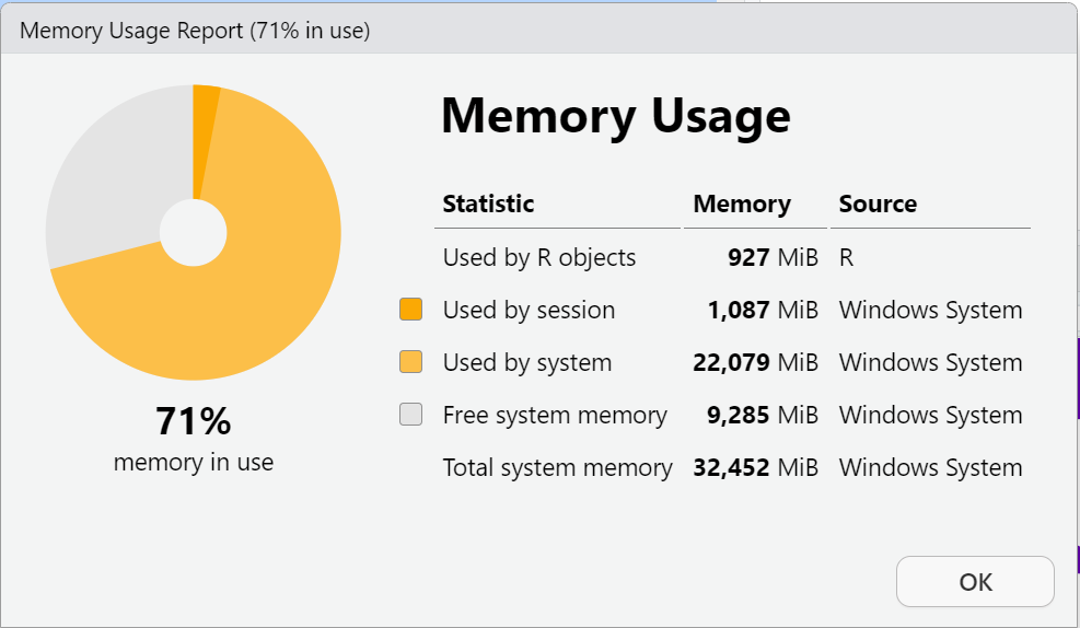
Run the following R code to load the PRAMS Phase 8 dataset into your R Session and check the “Global Environment”.
Here is my memory AFTER loading the PRAMS dataset into my “Global Environment”.
B. Save the data as a *.RData binary file for use in later analyses
One way to reduce the size of the PRAMS dataset is to save it as a native *.RData binary file format. So, let’s save the PRAMS dataset in this format on your computer.
# save the whole dataset as *.RData format
save(prams,
     file = "prams.RData")
On my computer, here is a comparison of the size of these 2 files:
-
phase8_arf_2016_2021.sas7bdatis 1,095,499,776 bytes (which is 1.02 GB) -
prams.RDatais only 34,713,319 (which is only 0.0323 GB)
This is a file size reduction of 96.83%!!
Now that we’ve reduced the file size of the dataset on your computer’s hard drive (or cloud storage), let’s also clear up the “Global Environment” back in your current RStudio computing session.
C. Clean up files to save memory
Now that we’ve saved the data, let’s remove the PRAMS data object from the RStudio session.
- For now we can simply remove everything using the
rm(list=ls()). - However, if you have other objects you want to keep, you can specifically only remove the PRAMS dataset using
rm(prams).
# remove all objects from Global Environment
rm(list=ls())

# confirm Global Environment is empty
# list all objects
ls()character(0)# and free any currently unused memory
gc() used (Mb) gc trigger (Mb) max used (Mb)
Ncells 2159105 115.4 4309787 230.2 4309787 230.2
Vcells 3931672 30.0 153079486 1168.0 112150029 855.7After we remove everything, let’s look at the session memory again.
Now let’s read the PRAMS data back in, but this time read in the prams.RData binary R data formatted file. We will use the built-in load() function.
# load back only the prams dataset
load(file = "prams.RData")
Let’s check the R session memory again:

I know this didn’t make a large difference for the R session available memory, but by doing this process:
- The PRAMS dataset now takes up less memory on your computer’s file storage, and
- The
load()function for theprams.RDatafile should run faster when beginning your R computing session instead of having to use thehavenpackage to read in the SAS formatted file everytime.
As a quick comparison on my computer (Windows 11), the time to read in the SAS formatted file was about 14 sec:
> system.time(
+   prams <-
+     read_sas("phase8_arf_2016_2021.sas7bdat")
+ )
   user  system elapsed
  13.44    0.47   13.96
And the time to read in the prams.RData file was only about 1.5 sec.
> system.time(
+   load("prams.RData")
+ )
   user  system elapsed
   1.45    0.08    1.54
2. Getting started with PRAMS Data
Breastfeeding summary - UNWEIGHTED data
Let’s look at whether the mother ever breastfed her baby - this is variable BF5EVER, where 1 = “NO” and 2 = “YES”.
For the UNWEIGHTED data, let’s get a simple table of breastfeeding by STATE (variable STATE) and YEAR (variable NEST_YR).
As we can see below, in 2017 for the state of GA, 919 women responded to this question:
- 919 women responded
- 170 said NO
- 749 said YES
- 36 were missing a response (indicated by
<NA>)
     BF5EVER.f
STATE   NO  YES <NA>
   AK   71  927   47
   AL  181  659   42
   CO   73 1037   18
   DE  126  728   37
   GA  170  749   36
   IA  136  867   30
   IL  140 1048   36
   KS   81  856   58
   KY  139  536   27
   LA  285  586   23
   MA  115 1268   40
   MD   97  928   35
   ME   88  754   30
   MI  290 1532   75
   MO  166  908   37
   MT   66  851   20
   ND  102  472   17
   NH   42  523   15
   NJ  125 1102   31
   NM  123 1038   19
   NY  109  706   33
   PA  164 1023   42
   PR   81  928   23
   RI  105  960   37
   SD  150  946   35
   UT   93 1305   49
   VA   88  969   26
   VT   54  780   14
   WA   69 1138   31
   WI  221 1051   74
   WV  186  475   38
   WY   49  438   16
   YC   99 1125   69
This aligns with the CDC PRAMS Indicators Report for GA in 2020 - scroll to the bottom to see the RAW count of 919 women who responded to “Ever Breastfed” in GA in 2017.
Breastfeeding summary - WEIGHTED data
In the CDC PRAMS Indicators Report for GA in 2020 the columns that have the 95% CI (confidence intervals) for the percentages are the population weighted percentage estimates for the Stats of GA during that year.
To get the estimated percentage of women in the stats of GA who had “ever breastfed” in 2017, we need to use the survey package and apply the proper sample weighting to get these estimates.
library(survey)

# Let's look at just GA to start with
# use dplyr to filter out just GA
prams_ga <- prams %>%
  filter(STATE == "GA")

# create the survey design file for GA
prams_ga.svy <-
  svydesign(ids = ~0, strata = ~SUD_NEST,
            fpc = ~TOTCNT, weights = ~WTANAL,
            data = prams_ga)

# get a table of ever breastfed
# by YEAR
svyby(~BF5EVER.f, ~NEST_YR,
      design = prams_ga.svy,
      svytotal, na.rm=TRUE)
NEST_YR BF5EVER.fNO BF5EVER.fYES se.BF5EVER.fNO se.BF5EVER.fYES
2017 2017 17639.96 101686.10 2045.415 2271.075
2018 2018 20187.62 98909.35 2151.496 2351.330
2019 2019 24099.04 95019.86 2273.415 2279.851
2020 2020 21827.55 94125.72 2209.745 2457.097
2021 2021 23724.68 93896.73 2266.811 2256.488From this we can see that the population estimates for 2017 are:
- Breastfed ever = NO: 17639.96 +/- 2045.415
- Breastfed ever = YES: 101686.10 +/- 2271.075
This leads to a percentage of YES estimate of 101686.10 * 100 / (101686.10 + 17639.96) = 85.2170096% which should match pretty closely to what is in the CDC PRAMS Indicators Report for GA in 2020.
We can also get the percentage of overall breastfeeding YES for the USA for the 40 “states” (technically 38 states, Puerto Rico, and New York City) that were included in the PRAMS dataset in 2020 (see the last column in the CDC report), using the following R code. Note: 2 “states” did not have data in 2020: Connecticut and Florida.
# get overall for 2020 - all states
# make survey design file
prams.svy <-
  svydesign(ids = ~0, strata = ~SUD_NEST,
            fpc = ~TOTCNT, weights = ~WTANAL,
            data = prams)

svyby(~BF5EVER.f, ~NEST_YR,
      design = prams.svy,
      svytotal, na.rm=TRUE)
NEST_YR BF5EVER.fNO BF5EVER.fYES se.BF5EVER.fNO se.BF5EVER.fYES
2016 2016 187666.4 1324171 4398.541 4798.836
2017 2017 208863.1 1497127 4762.339 5452.232
2018 2018 242991.5 1716913 5220.222 5979.598
2019 2019 236841.9 1680987 5404.761 6877.697
2020 2020 225560.3 1609464 4884.871 5540.240
2021 2021 212618.8 1521303 5196.234 6058.572From this we can see that the population estimates for the “whole USA” for 2020 were:
- Breastfed ever = NO: 225560.3 +/- 4884.871
- Breastfed ever = YES: 1609464 +/- 5540.240
This leads to a percentage of YES estimate of 1609464 * 100 / (1609464 + 225560.3) = 87.7080483% which is pretty close to what is in the CDC PRAMS Indicators Report for GA in 2020 - with some numerical precision variation due to software algorithms.
Congratulations on getting started with the PRAMS Dataset
3. Data Wrangling with PRAMS
Data wrangling with the PRAMS data isn’t much different from the methods already covered in Module 1.3.2.
The code below shows an example of recoding the VITAMIN variable from PRAMS.
# create a factor variable
# and add labels
prams$VITAMIN.f <- factor(
  prams$VITAMIN,
  levels = c(1, 2, 3, 4),
  labels = c("1 = DIDNT TAKE VITAMIN",
             "2 = 1-3 TIMES/WEEK",
             "3 = 4-6 TIMES/WEEK",
             "4 = EVERY DAY/WEEK")
)

# create variable for anyone who
# took vitamins 4+ times a week
prams$VITAMIN_4plus <-
  ifelse(prams$VITAMIN > 2, 1, 0)

# add labels, make a factor
prams$VITAMIN_4plus.f <- factor(
  prams$VITAMIN_4plus,
  levels = c(0, 1),
  labels = c("3x/week or less",
             "4x/week or more")
)

# get stats for 2020 for GA
prams %>%
  filter(NEST_YR == 2020) %>%
  filter(STATE == "GA") %>%
  with(., table(STATE, VITAMIN_4plus.f,
                useNA = "ifany"))
VITAMIN_4plus.f
STATE 3x/week or less 4x/week or more <NA>
GA 443 247 2Get table of weighted percentages for “Taking Multivitamin 4+/week” for GA by Year.
# get a table of vitamins 4+ times per week
# by YEAR
svyby(~VITAMIN_4plus.f, ~NEST_YR,
      design = prams_ga.svy,
      svytotal, na.rm=TRUE)
NEST_YR VITAMIN_4plus.f3x/week or less VITAMIN_4plus.f4x/week or more
2017 2017 86492.91 37312.18
2018 2018 76796.28 43028.81
2019 2019 74523.87 46236.67
2020 2020 75313.80 42263.67
2021 2021 69861.41 48766.71
se.VITAMIN_4plus.f3x/week or less se.VITAMIN_4plus.f4x/week or more
2017 2715.819 2653.349
2018 2817.611 2732.988
2019 2786.899 2666.692
2020 2779.229 2802.984
2021 2824.624 2693.566The unweighted breakdown for GA in 2020
- NO Vitamins =< 3x/wk 443 64.2%
- YES Vitamins => 4x/wk 247 35.8%
- Total 690
Weighted Breakdown for GA in 2020
- NO Vitamins =< 3x/wk 75313.80 +/- 2779.229 (64.1%) []
- YES Vitamins => 4x/wk 42263.67 +/- 2802.984 (35.9%) [33.6%, 38.3%]
- Total 117,577.47
Get Proportions and 95% Confidence Intervals
prams_ga2000 <- prams %>%
  filter(STATE == "GA") %>%
  filter(NEST_YR == 2020)

# create the survey design file for GA
# for year 2020
prams_ga2000.svy <-
  svydesign(ids = ~0, strata = ~SUD_NEST,
            fpc = ~TOTCNT, weights = ~WTANAL,
            data = prams_ga2000)

svytable(~VITAMIN_4plus,
         prams_ga2000.svy)
VITAMIN_4plus
0 1
75313.80 42263.67 svyciprop(~VITAMIN_4plus,
prams_ga2000.svy,
na.rm = T) 2.5% 97.5%
VITAMIN_4plus 0.359 0.315 0.407Compare the results below to the EXCEL spreadsheet Pregnancy Risk Assessment Monitoring System (PRAMS) MCH Indicators (standard version) - see 2020 for GA - 1st set of indicators for Vitamins taken 4x a week or more.
The code below adds custom code for computing the confidence intervals with the survey-weighted dataset.
prams_ga2000 <- prams %>%
  filter(STATE == "GA") %>%
  filter(NEST_YR == 2020)

# create the survey design file for GA
# for year 2020
prams_ga2000.svy <-
  svydesign(ids = ~0, strata = ~SUD_NEST,
            fpc = ~TOTCNT, weights = ~WTANAL,
            data = prams_ga2000)

# get a table of vitamins 4+ times per week
# by YEAR
svyby(~VITAMIN_4plus.f, ~NEST_YR,
      design = prams_ga2000.svy,
      svytotal, na.rm=TRUE)
NEST_YR VITAMIN_4plus.f3x/week or less VITAMIN_4plus.f4x/week or more
2020 2020 75313.8 42263.67
se.VITAMIN_4plus.f3x/week or less se.VITAMIN_4plus.f4x/week or more
2020 2779.229 2802.984# add custom statistic forconfidence intervals
confidence_intervals <- function(data, variable, by, ...) {
## extract the confidence intervals and multiply to get percentages
props <- svyciprop(as.formula(paste0( "~" , variable)),
data, na.rm = TRUE)
## extract the confidence intervals
as.numeric(confint(props) * 100) %>% ## make numeric and multiply for percentage
round(., digits = 1) %>% ## round to one digit
c(.) %>% ## extract the numbers from matrix
paste0(., collapse = "-") ## combine to single character
}
library(gtsummary)
tbl_svysummary(
data = prams_ga2000.svy,
include = c(VITAMIN_4plus),
statistic = list(everything() ~ c("{n} ({p}%)"))
) %>%
add_n() %>%
add_stat(fns = everything() ~ confidence_intervals) %>%
modify_header(
list(
n ~ "**Weighted total (N)**",
stat_0 ~ "**Weighted Count**",
add_stat_1 ~ "**95%CI**"
))| Characteristic | Weighted total (N) | Weighted Count1 | 95%CI |
|---|---|---|---|
| VITAMIN_4plus | 117,577 | 42,264 (36%) | 31.5-40.7 |
| Unknown | 363 | ||
| 1 n (%) | |||
4. Visualizing PRAMS Data
Examples will be posted here for making graphs and figures with suggestions on handling very large datasets.
let’s look at maternal age variable MAT_AGE_PU, see PRAMS Codebook.
Histogram of Maternal Age - Unweighted
hist(prams$MAT_AGE_PU)
Histogram of Maternal Age - Complex Survey Weighted
# use survey design data
# get histogram using svyhist() function
svyhist(formula = ~MAT_AGE_PU,
        design = prams.svy)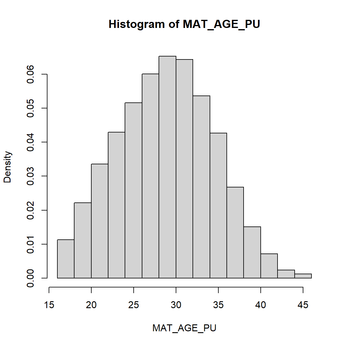
Histogram of Maternal weight gain in lbs - Unweighted Data
# MOMLBS
hist(prams$MOMLBS,
     main = "Histogram of Unweighted Data")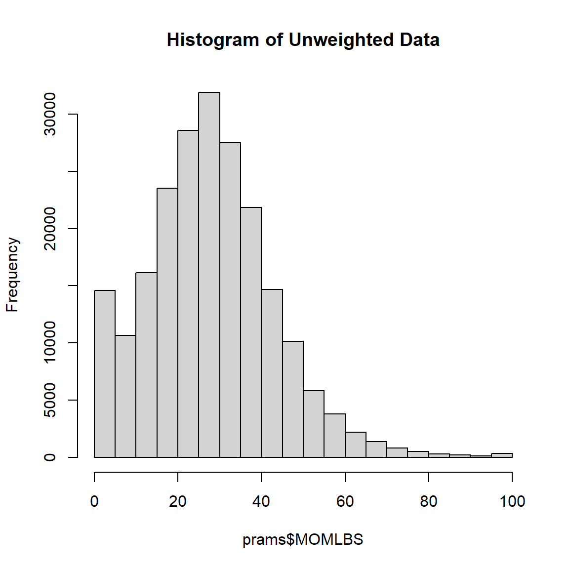
Summary statistics of Unweighted Data
summary(prams$MOMLBS) Min. 1st Qu. Median Mean 3rd Qu. Max. NAs
0.00 19.00 28.00 28.48 37.00 97.00 6275 Histogram of Maternal weight gain in lbs - Complex Survey Weighted Data
svyhist(formula = ~MOMLBS,
        design = prams.svy)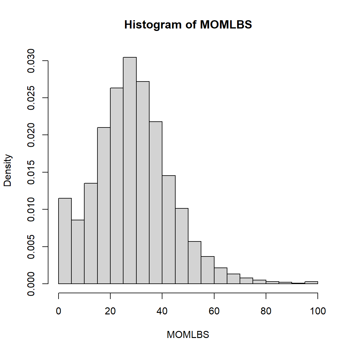
Scatterplot of Weight Gain by Age - Unweighted Data
Look at GA for 2020
library(ggplot2)
ggplot(prams_ga2000, aes(x=MAT_AGE_PU, y=MOMLBS)) +
  geom_point()
Weighted plot - notice the varying sizes of the dots (bubbles)
svyplot(MOMLBS~MAT_AGE_PU,
        prams_ga2000.svy,
        style = "bubble")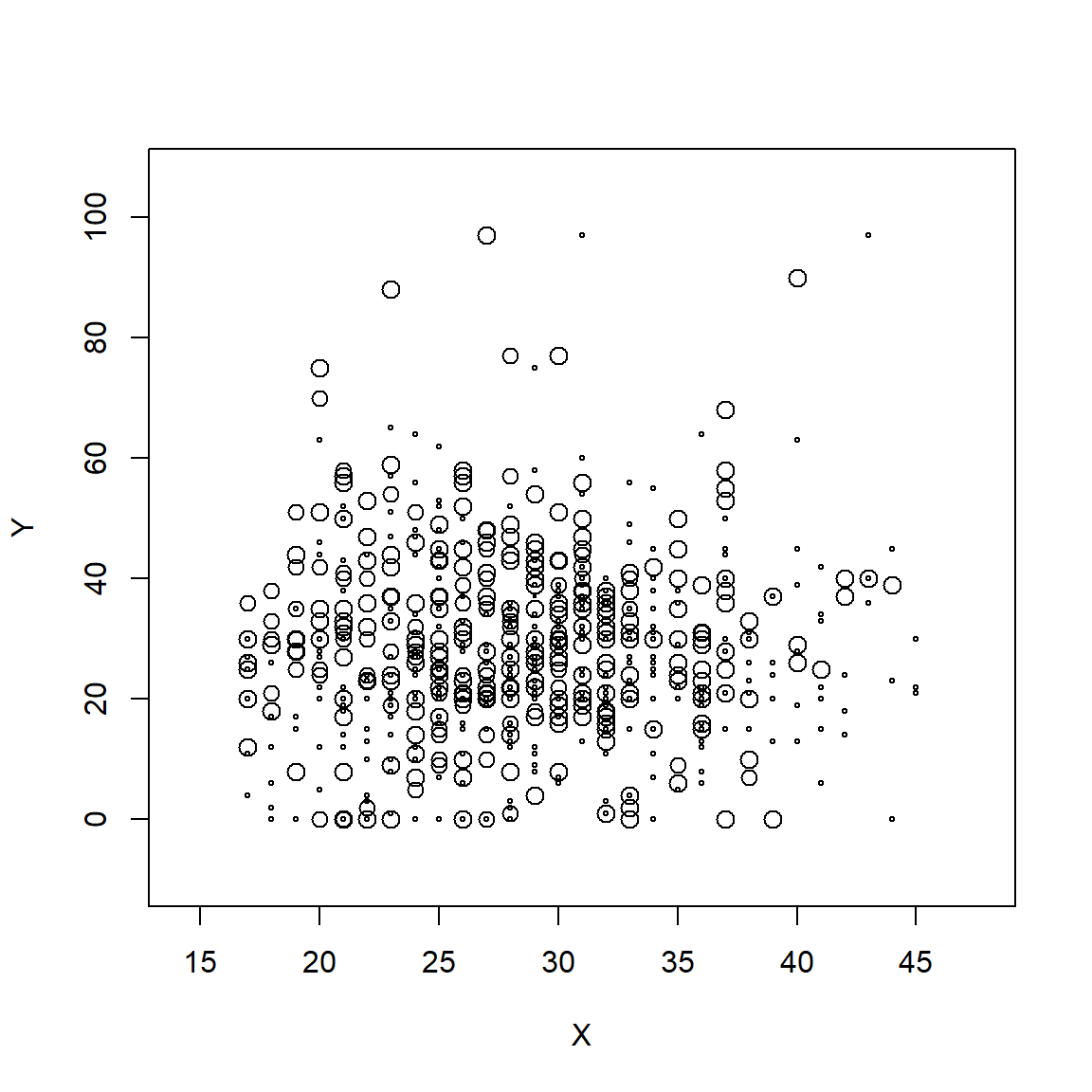
Another option - gray scale hex symbols - darker indicate higher counts, see help(svyplot, package = "survey").
svyplot(MOMLBS~MAT_AGE_PU,
        prams_ga2000.svy,
        style = "grayhex")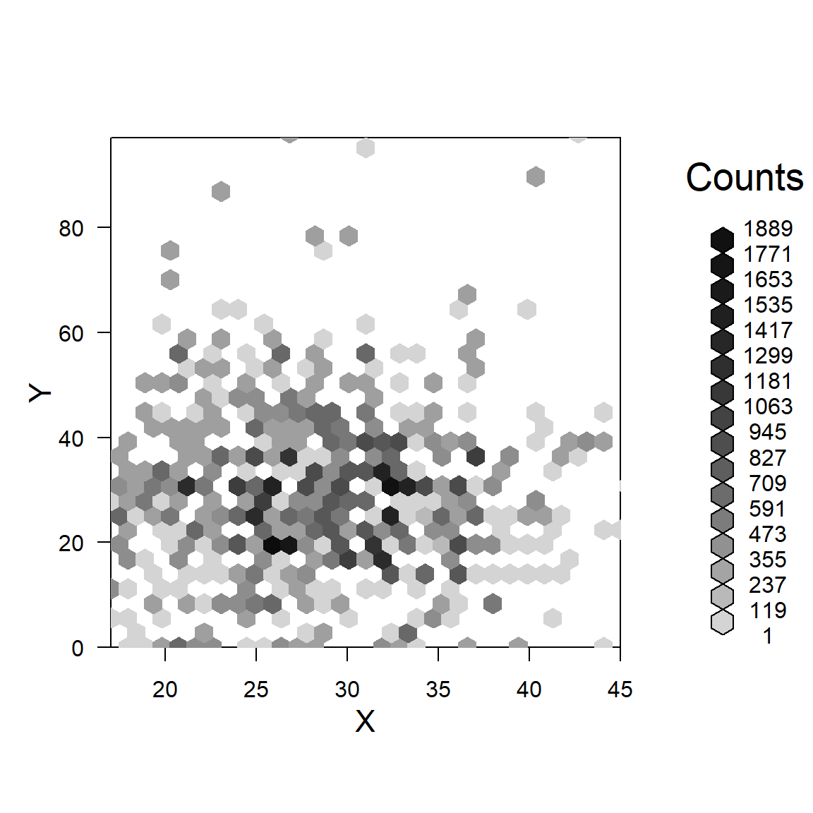
5. Missing Data in PRAMS
Let’s look at the missing data for the VITAMIN variable for GA in 2020.
prams_ga2000 <- prams %>%
  filter(STATE == "GA") %>%
  filter(NEST_YR == 2020)

# amount of missing data for VITAMIN
# unweighted
 #   1    2    3    4 <NA>
 # 390   53   33  214    2
# 2/692 = 0.289%
table(prams_ga2000$VITAMIN, useNA = "ifany")
   1    2    3    4 <NA>
 390   53   33  214    2
This is areallysmall amount - only 2 NAs - but this is much larger in the weighted sample.
Create a missing value indicator variable for VITAMIN and look at the amounts in the weighted sample.
The amount is still small but the range in the weighted sample shown below is informative.
# add missing indicator for VITAMIN
prams_ga2000$VITAMIN_na <-
  as.numeric(is.na(prams_ga2000$VITAMIN))
sum(prams_ga2000$VITAMIN_na)
[1] 2# create the survey design file for GA
# for year 2020
prams_ga2000.svy <-
svydesign(ids = ~0, strata = ~SUD_NEST,
fpc = ~TOTCNT, weights = ~WTANAL,
data = prams_ga2000)
tbl_svysummary(
data = prams_ga2000.svy,
include = c(VITAMIN_na),
statistic = list(everything() ~ c("{n} ({p}%)"))
) %>%
add_n() %>%
add_stat(fns = everything() ~ confidence_intervals) %>%
modify_header(
list(
n ~ "**Weighted total (N)**",
stat_0 ~ "**Weighted Count**",
add_stat_1 ~ "**95%CI**"
)) | Characteristic | Weighted total (N) | Weighted Count1 | 95%CI |
|---|---|---|---|
| VITAMIN_na | 117,940 | 363 (0.3%) | 0.1-1.8 |
| 1 n (%) | |||
# weighted 0.3%, CI: 0.1 to 1.8%6. PRAMS Statistical Tests and Models
Linear Regression Example
Association of age and weight gain using linear regression - Unweighted model
Call:
lm(formula = MOMLBS ~ MAT_AGE_PU, data = prams_ga2000)

Residuals:
    Min      1Q  Median      3Q     Max
-29.566  -8.733  -1.089   8.161  68.722

Coefficients:
            Estimate Std. Error t value Pr(>|t|)
(Intercept) 26.23389    2.80325   9.358   <2e-16 ***
MAT_AGE_PU   0.07572    0.09545   0.793    0.428
---
Signif. codes:  0 '***' 0.001 '**' 0.01 '*' 0.05 '.' 0.1 ' ' 1

Residual standard error: 15.18 on 686 degrees of freedom
  (4 observations deleted due to missingness)
Multiple R-squared:  0.0009166, Adjusted R-squared:  -0.0005398
F-statistic: 0.6294 on 1 and 686 DF,  p-value: 0.4279
Association of age and weight gain using linear regression - Weighted model
Call:
svyglm(formula = MOMLBS ~ MAT_AGE_PU, design = prams_ga2000.svy)

Survey design:
svydesign(ids = ~0, strata = ~SUD_NEST, fpc = ~TOTCNT, weights = ~WTANAL,
    data = prams_ga2000)

Coefficients:
             Estimate Std. Error t value Pr(>|t|)
(Intercept) 30.210104   3.935380   7.677 5.65e-14 ***
MAT_AGE_PU  -0.005842   0.135304  -0.043    0.966
---
Signif. codes:  0 '***' 0.001 '**' 0.01 '*' 0.05 '.' 0.1 ' ' 1

(Dispersion parameter for gaussian family taken to be 231.9695)

Number of Fisher Scoring iterations: 2
Contingency tables and Chi-square test - vitamin use by breastfeeding - Unweighted Data
table(prams_ga2000$VITAMIN_4plus.f,
      prams_ga2000$BF5EVER.f,
      useNA = "ifany")
                   NO YES <NA>
  3x/week or less  95 337   11
  4x/week or more  18 225    4
<NA> 1 1 0library(gmodels)
CrossTable(x = prams_ga2000$VITAMIN_4plus.f,
y = prams_ga2000$BF5EVER.f,
expected = TRUE,
prop.r = FALSE,
prop.c = TRUE,
prop.t = FALSE,
prop.chisq = FALSE,
chisq = TRUE,
format = "SPSS")
   Cell Contents
|-------------------------|
|                   Count |
|         Expected Values |
|          Column Percent |
|-------------------------|

Total Observations in Table:  675

                             | prams_ga2000$BF5EVER.f
prams_ga2000$VITAMIN_4plus.f |       NO  |      YES  | Row Total |
-----------------------------|-----------|-----------|-----------|
             3x/week or less |       95  |      337  |      432  |
                             |   72.320  |  359.680  |           |
                             |   84.071% |   59.964% |           |
-----------------------------|-----------|-----------|-----------|
             4x/week or more |       18  |      225  |      243  |
                             |   40.680  |  202.320  |           |
                             |   15.929% |   40.036% |           |
-----------------------------|-----------|-----------|-----------|
                Column Total |      113  |      562  |      675  |
                             |   16.741% |   83.259% |           |
-----------------------------|-----------|-----------|-----------|


Statistics for All Table Factors


Pearson's Chi-squared test
------------------------------------------------------------
Chi^2 =  23.72972     d.f. =  1     p =  1.108573e-06

Pearson's Chi-squared test with Yates' continuity correction
------------------------------------------------------------
Chi^2 =  22.69497     d.f. =  1     p =  1.898642e-06


       Minimum expected frequency: 40.68
Contingency tables and Chi-square test - vitamin use by breastfeeding - Unweighted Data
svytable(~VITAMIN_4plus.f + BF5EVER.f,
         prams_ga2000.svy)
BF5EVER.f
VITAMIN_4plus.f NO YES
3x/week or less 18458.169 55008.856
4x/week or more 3334.398 38789.322svychisq(~VITAMIN_4plus.f + BF5EVER.f,
prams_ga2000.svy,
statistic = "Chisq")
    Pearson's X^2: Rao & Scott adjustment

data:  svychisq(~VITAMIN_4plus.f + BF5EVER.f, prams_ga2000.svy, statistic = "Chisq")
X-squared = 31.025, df = 1, p-value = 1.222e-05
Logistic Regression Example
Let’s look at multi-vitamin use 4x/week by breastfeeding and maternal age.
Unweighted Logistic Regression Results
glm1 <-glm(VITAMIN_4plus ~ MAT_AGE_PU + BF5EVER.f,
           data = prams_ga2000,
           family = "binomial")
gtsummary::tbl_regression(glm1,
exponentiate = TRUE)| Characteristic | OR | 95% CI | p-value |
|---|---|---|---|
| Maternal age grouped | 1.07 | 1.04, 1.11 | <0.001 |
| BF5EVER.f | |||
| NO | — | — | |
| YES | 2.82 | 1.67, 4.99 | <0.001 |
| Abbreviations: CI = Confidence Interval, OR = Odds Ratio | |||
Weighted Logistic Regression Results
wtglm1 <- svyglm(VITAMIN_4plus ~ MAT_AGE_PU + BF5EVER.f,
                 design = prams_ga2000.svy,
                 family=quasibinomial())
summary(wtglm1)
Call:
svyglm(formula = VITAMIN_4plus ~ MAT_AGE_PU + BF5EVER.f, design = prams_ga2000.svy,
    family = quasibinomial())

Survey design:
svydesign(ids = ~0, strata = ~SUD_NEST, fpc = ~TOTCNT, weights = ~WTANAL,
    data = prams_ga2000)

Coefficients:
             Estimate Std. Error t value Pr(>|t|)
(Intercept)  -3.36672    0.60317  -5.582 3.46e-08 ***
MAT_AGE_PU    0.06250    0.01901   3.287 0.001064 **
BF5EVER.fYES  1.18775    0.33359   3.561 0.000396 ***
---
Signif. codes:  0 '***' 0.001 '**' 0.01 '*' 0.05 '.' 0.1 ' ' 1

(Dispersion parameter for quasibinomial family taken to be 1.006803)

Number of Fisher Scoring iterations: 4 (Intercept) MAT_AGE_PU BF5EVER.fYES
0.0345025 1.0644955 3.2797036 7. PRAMS Reproducible Research Report
Here is an example Rmarkdown analysis report provided as a template to “kick start” your research with the PRAMS dataset.
- Download this Rmarkdown template PRAMS Rmarkdown Report.
- Knit to HTML PRAMS Report in HTML.
- Knit to DOC PRAMS Report in DOCX.
- Knit to PDF (if you’ve installed
tinytexpackage) PRAMS Report in PDF. - Knit with Parameters - Change the year from 2020 to 2018 and re-knit the document