5 + 5[1] 10(Asynchronous-Online)
When you download R from CRAN and install it on your computer, there is an R application that you can run. However, it is very bare bones. Here is a screenshot of what it looks like on my computer (Windows 11 operating system).
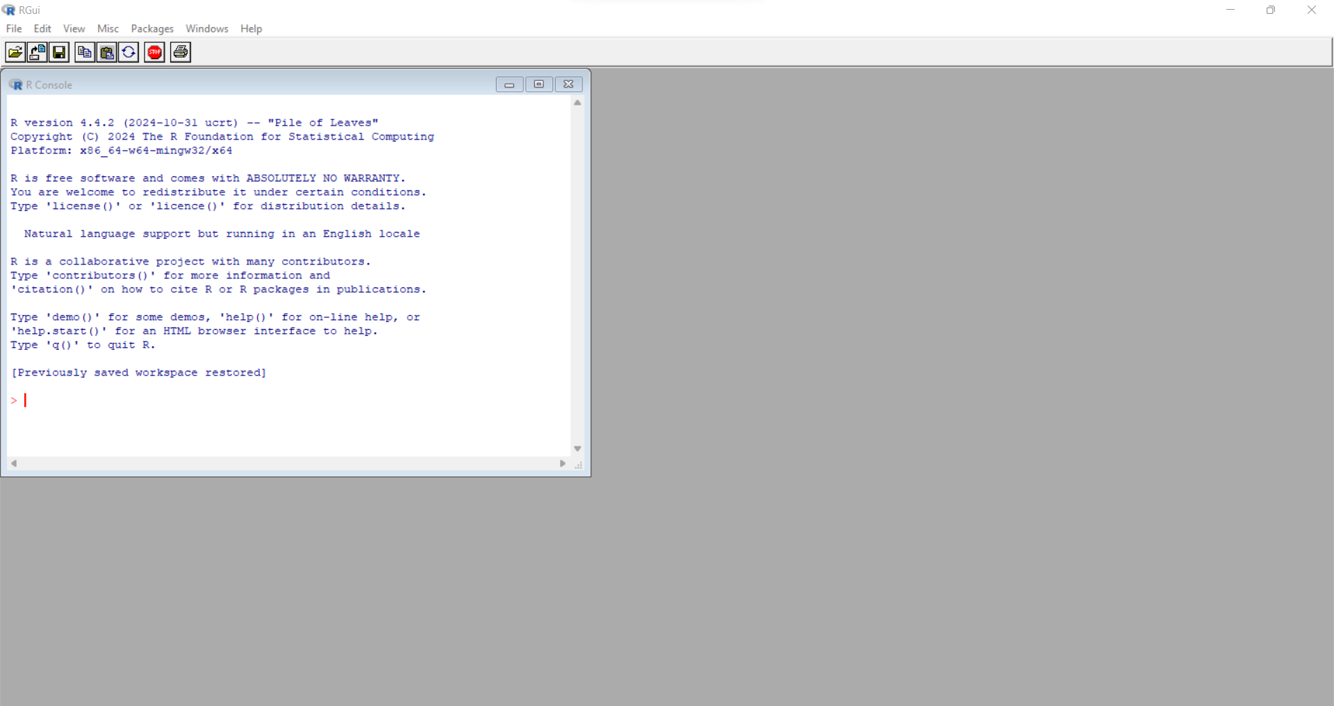
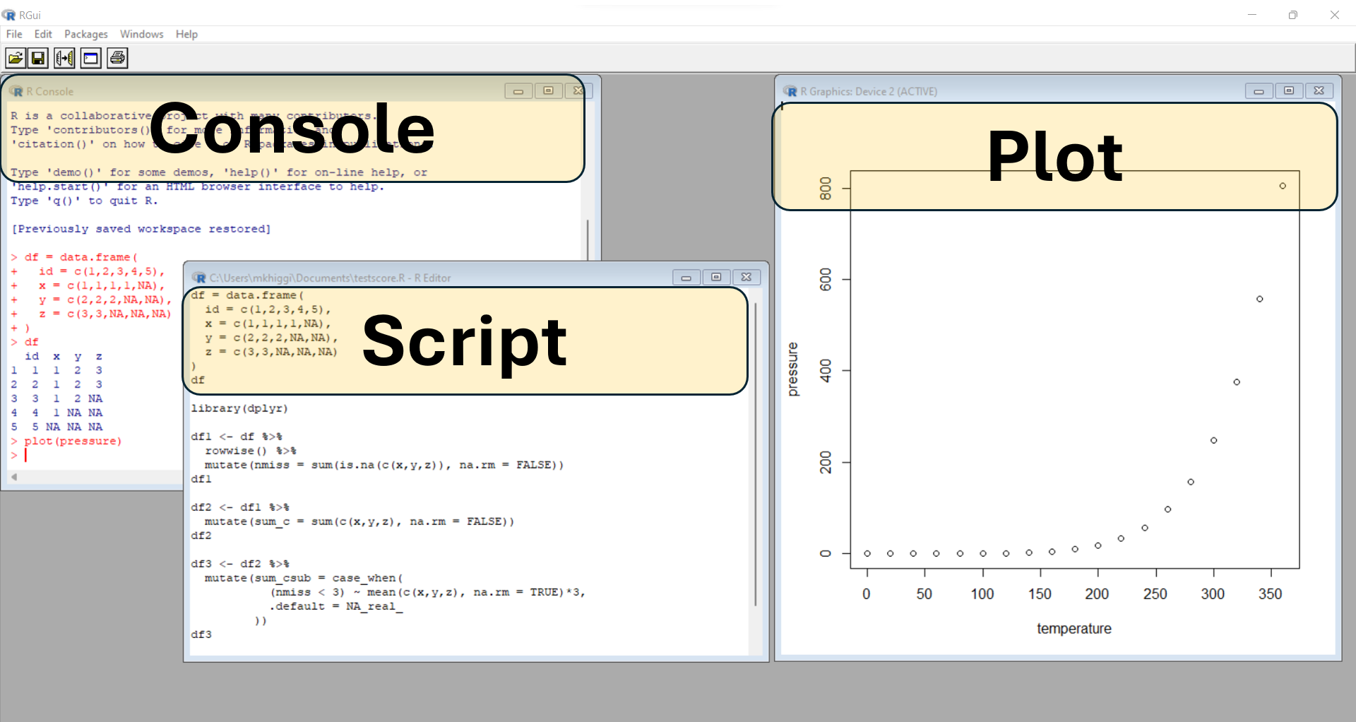
You can type commands in the console window at the prompt “>” but this is slow and tedious. You can also write and execute scripts from inside this application and see the output back in the console window as well as creating plots. But managing large projects using this interface is not efficient.
RStudio was founded in 2009 https://posit.co/about/ when it published the “free and open source” RStudio software. But over time, the RStudio application has expanded beyond just being used for the R programming language. You can now use RStudio for writing and managing projects with Python code, Markdown, LaTeX, Cascading Style Sheets and more.
So, in 2022, RStudio the company became Posit https://posit.co/blog/rstudio-is-becoming-posit/ to encompass the broader computing community.
The RStudio Integrated Development Environment (IDE) application provides much better tools for managing files within a given “project”. This biggest advantage of working in an IDE is everything is contained and managed within a given project, which is linked to a specific folder (container) on your computer (or cloud drive you may have access to).
However, you will still need to write and execute code using scripts and related files. An IDE is NOT a GUI (graphical user interface) which is the “point and click” workflow you may have experience with if you’ve used other analysis software applications such as SPSS, SAS Studio, Excel and similar.
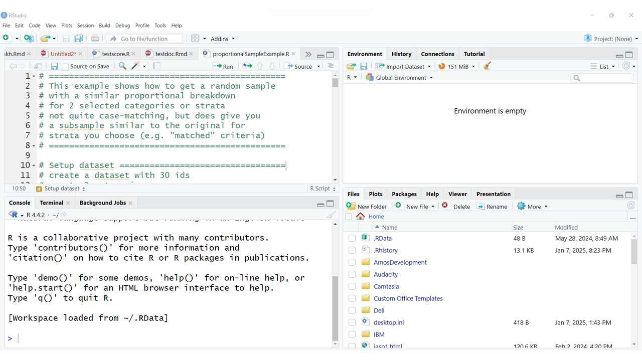
The interface is usually arranged with the following 4 “window panes”:
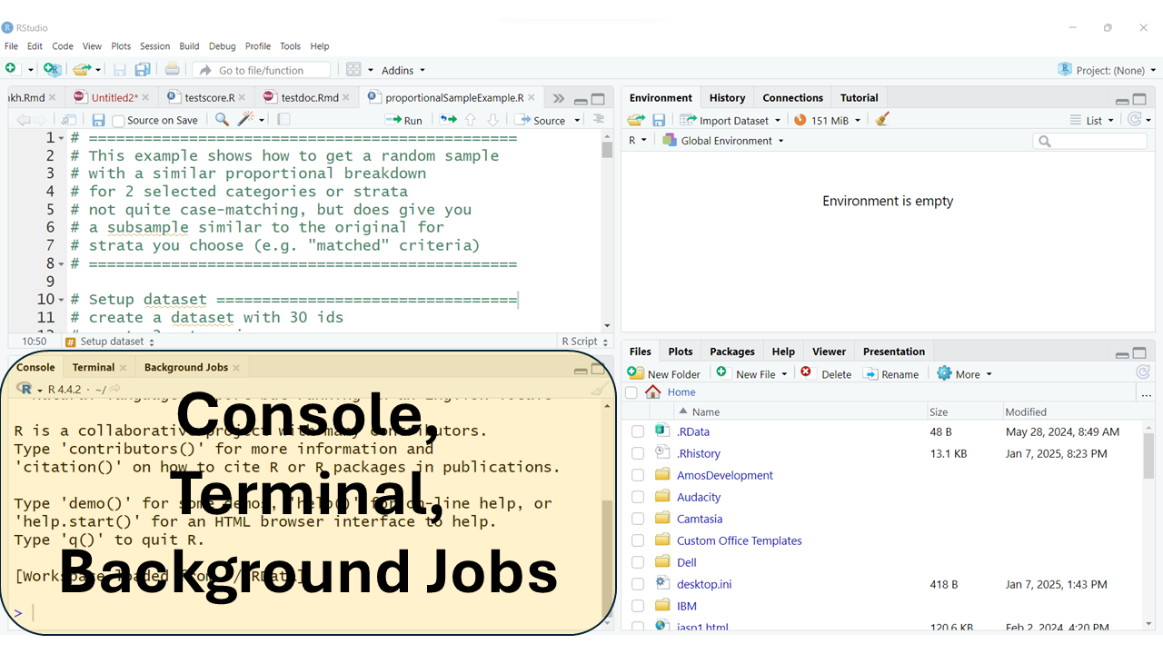
The typical arrangement, usually has the “Console” window pane at the bottom left. This window also usually has TABs for the “Terminal” and any “Background Jobs” that might be running.
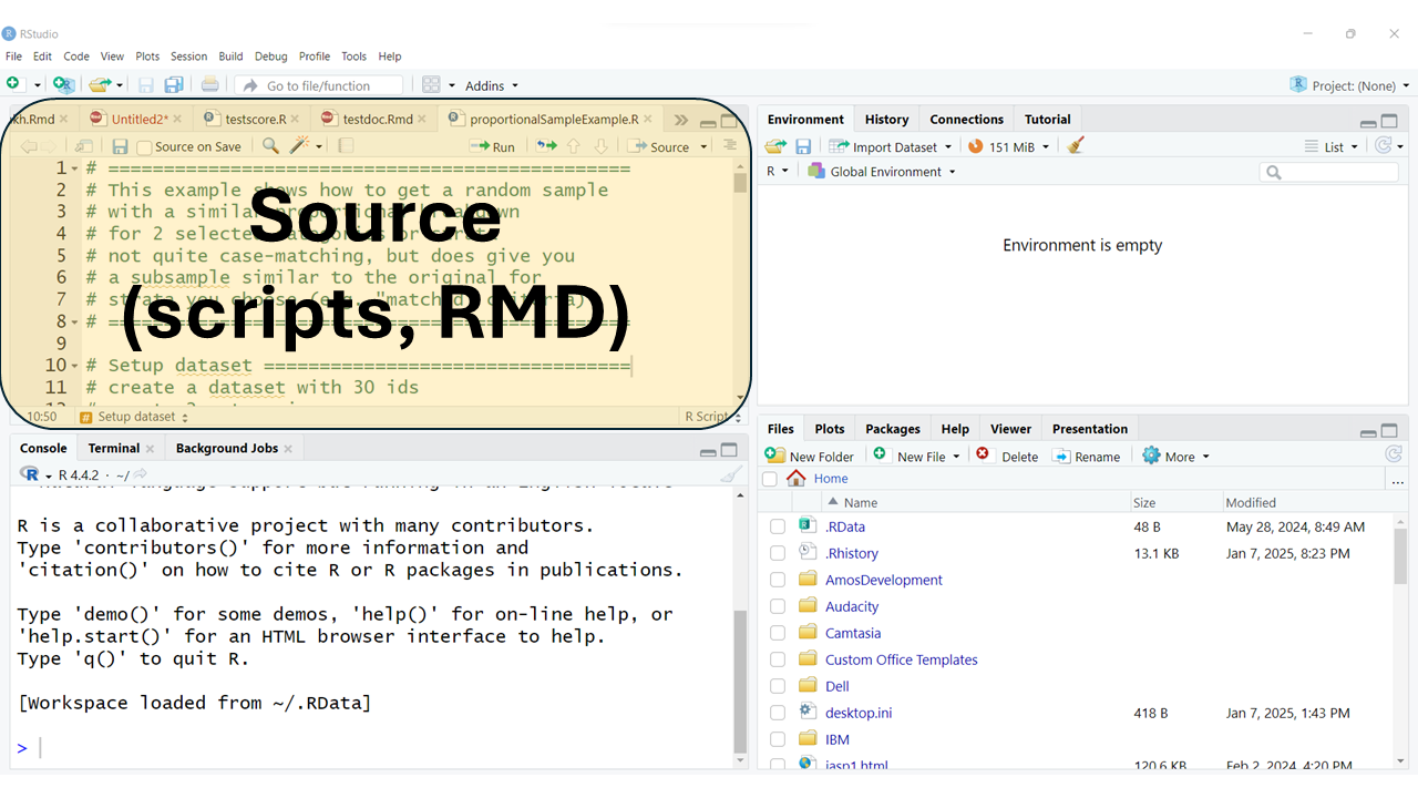
The “Source” window pane is usually at the top left. This is where you will do most of your editing of your R program scripts (*.R) or Rmarkdown files (*.Rmd). This is also where the data viewer window will open. You can also open and edit other kinds of files here as well (*.tex, *.css, *.txt, and more).
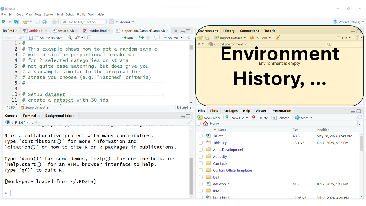
The top right window pane should always have your “Environment”, “History” and “Tutorial” TABs but may also have TABs for “Build” and “Git” and others depending on your project type and options selected.
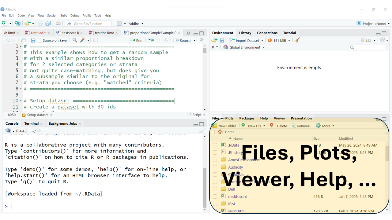
The bottom right window pane has TABs for your:
You also have the option to rearrange your window panes as well as change the look and feel of your programming interface and much more. To explore all of your options, click on the menu at the top for “Tools/Global Options”:
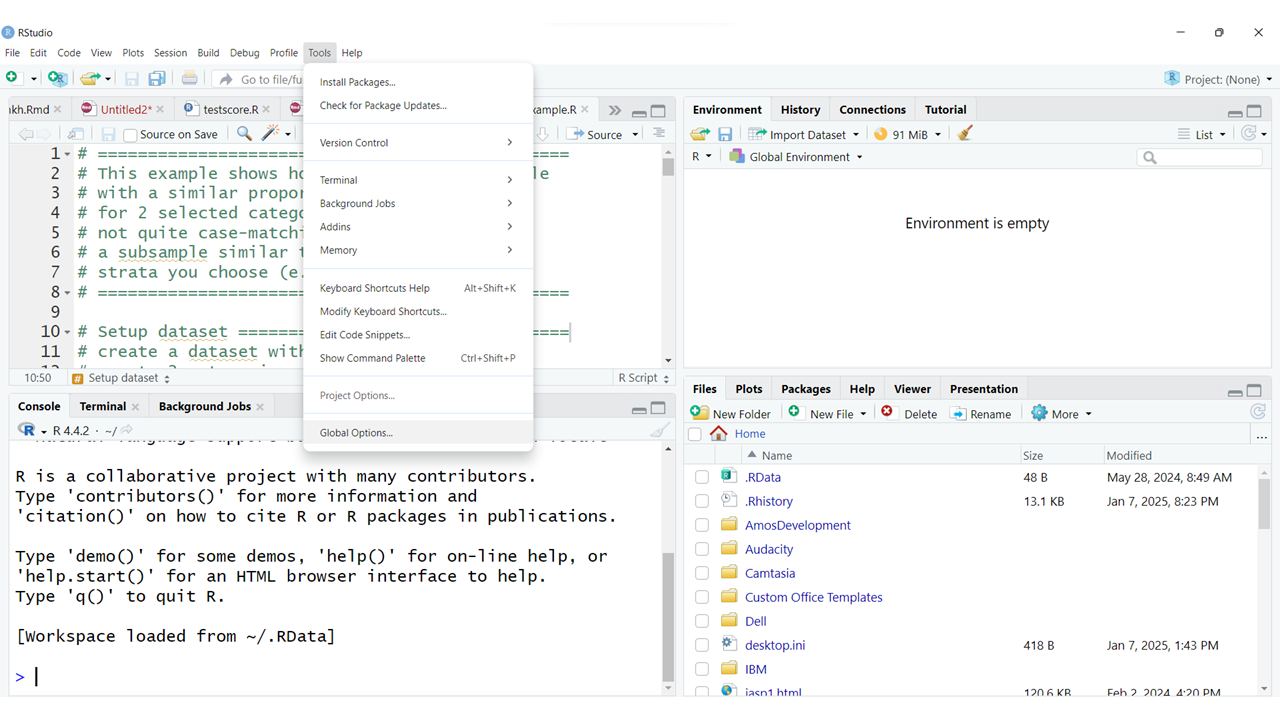
Take a look at the left side for the list of all of the options. Some of the most useful options to be aware of are:
In the “General” TAB is where you can see and confirm that R is installed and where the R programming language executable is installed on your computer.
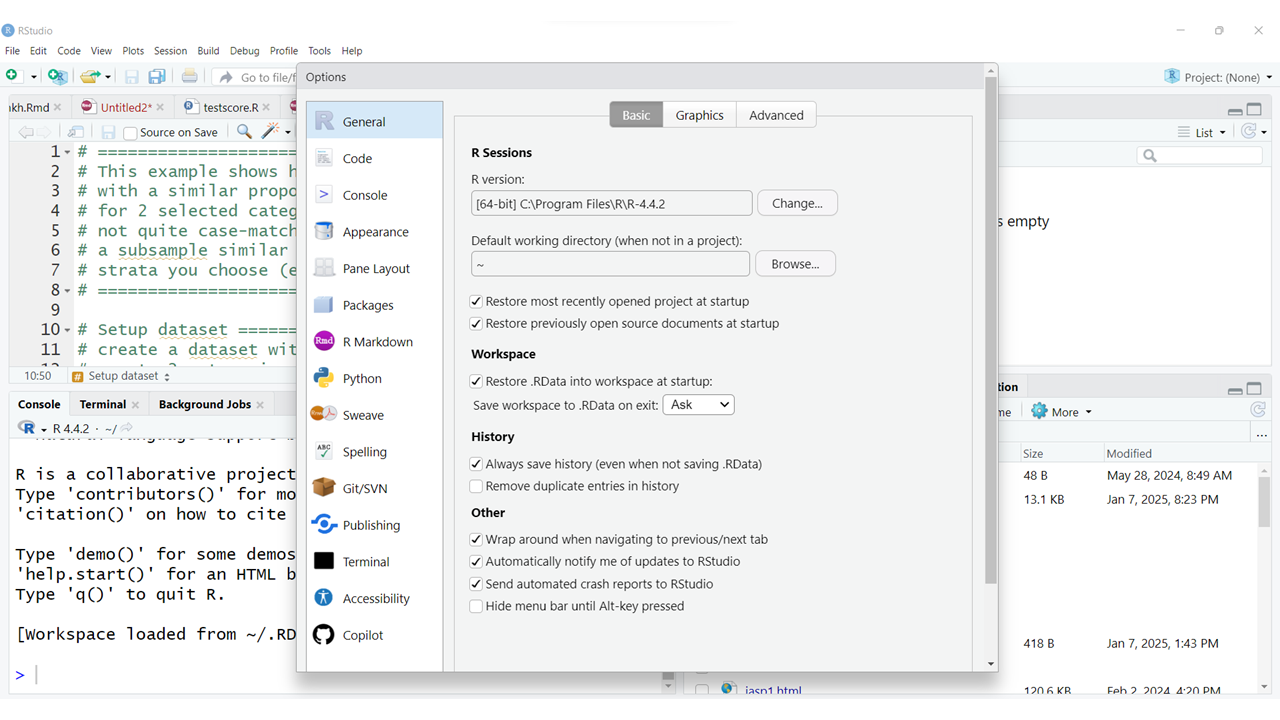
You will probably want to explore fine-tuning these parameters to customize the appearance of your RStudio preferences. For example, you can change the ZOOM level to improve readability. You may also want to change the FONT sizes for the Editor and Help windows as needed.
When making changes to your RStudio interface appearance, be aware that ZOOM and FONT size settings work together, so you may need to play around with the settings that work best for your monitor or device you are using.
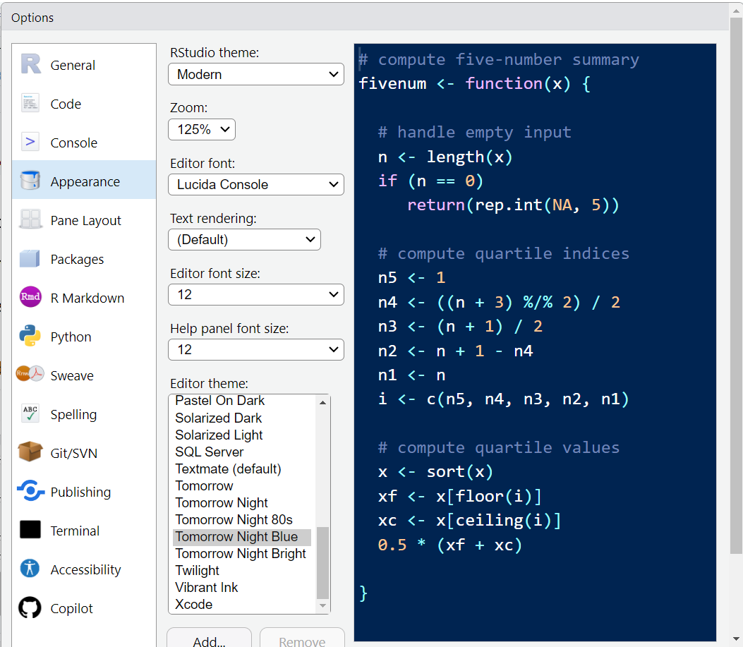
I also encourage you to try out different “Editor Themes” which will change the colors of the R code as well as background colors (light or dark).
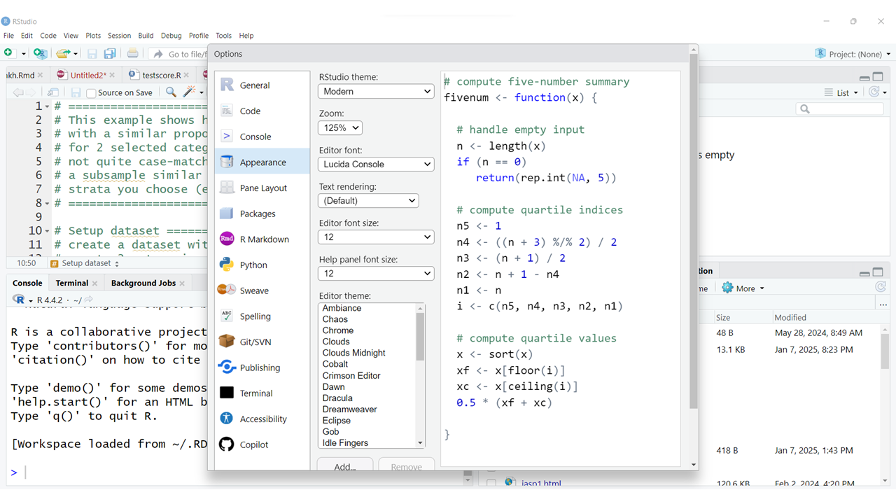
The default “Editor Theme” is textmate.
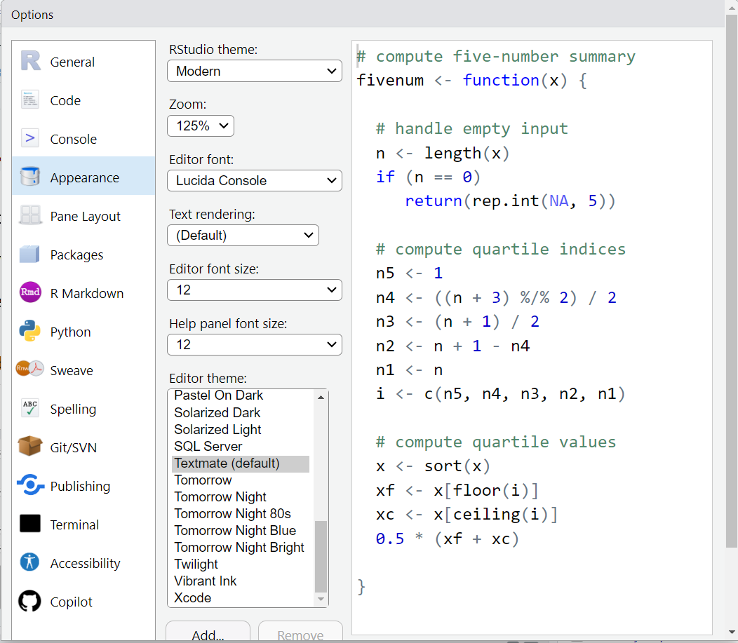
But here is an example of changing the theme to “Tomorrow Night Blue”.
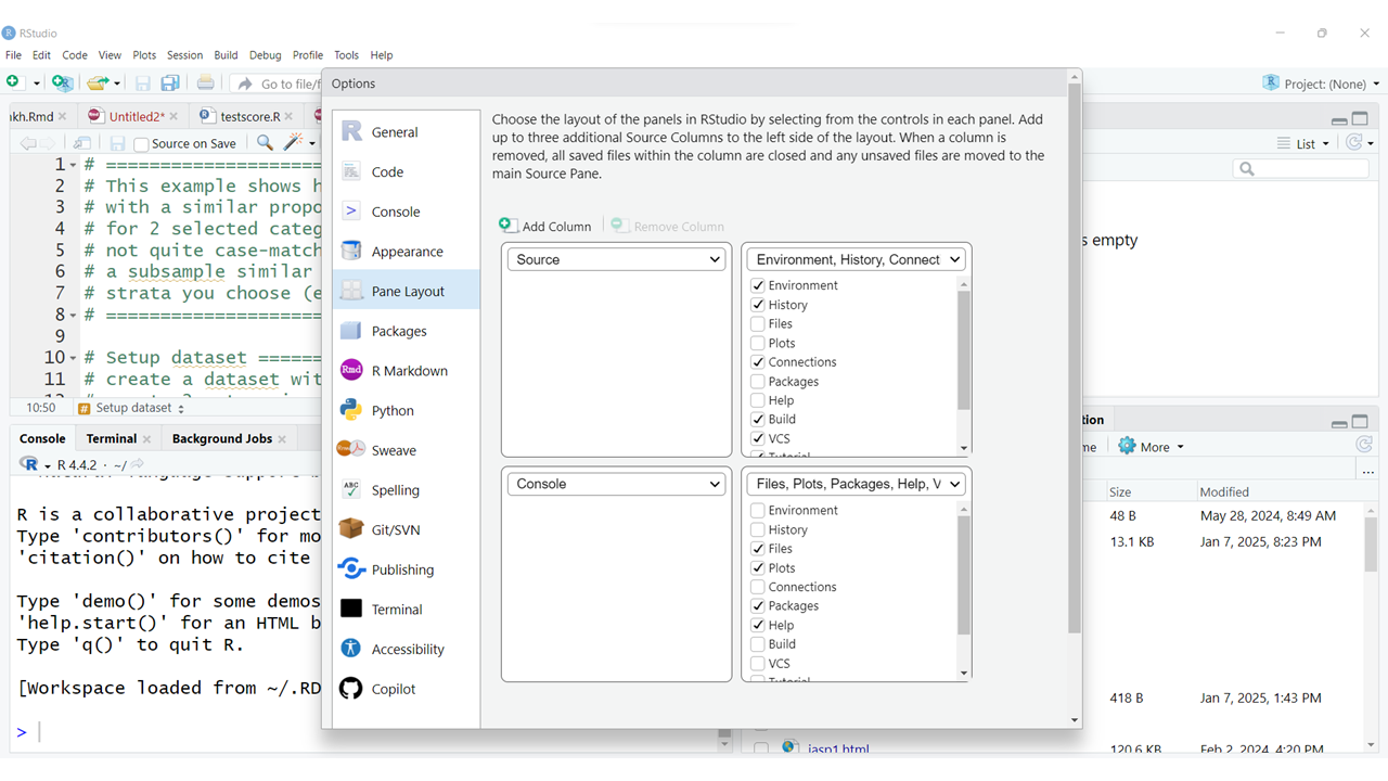
I would also suggest NOT changing the layout of the window panes until you are very familiar with the default settings. But in “Pane Layout” is where you can see what the default layout settings are and what other options are available to you.
So, let’s start with some simple R code using the Console window and typing commands at the > prompt (which is the greater than symbol).
You can write simple math expressions like 5 + 5.
5 + 5[1] 10Notice that the output shows the number 1 enclosed in square brackets [] followed by the answer (or output) of 10.
This is because R performed the addition operation using the + operator and then “saved” the output in temporary memory as a scalar object with 1 element, which is the number 10.
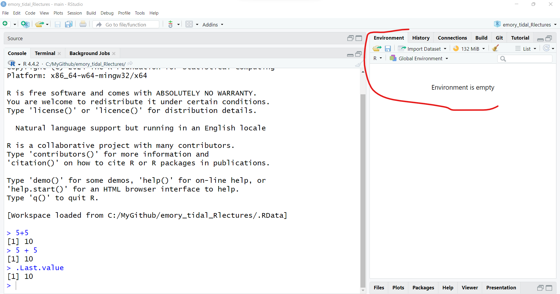
You can actually see this temporary object by typing .Last.value - which is only temporary and will be overwritten after the execution of the next R command.
.Last.value
[1] 10
However, if we look at our current computing environment (see “Global Environment” upper right window pane), it is still showing as empty.
This is because we have not yet “saved” the output into an object that we created. Let’s save the output from 5 + 5 into an object called ten.
To do this we need to do 2 things:
ten by<- to take the result of 5 + 5 and move it (save it or pipe it) into the object ten.ten <- 5 + 5<-?
The “R” language is actually a derivative of the original “S” language which stood for the “language of statistics” - it was written by statisticians for statisticians (and now data scientists). The original S language was written in the mid-1970’s by programmers/statisticians at Bell Labs/AT&T.
The <- actually comes from the physical key on their “APL” keyboards, for the APL programming language they were using at Bell Labs.
To “see” the output of this object called ten - you can either see it now in your Global Environment or type the object name in the Console to view it.
ten[1] 10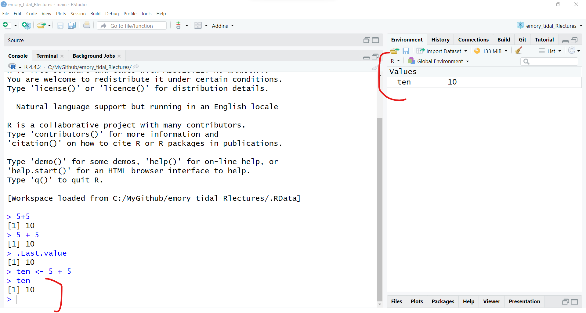
It is important to remember that R is an “object-oriented” programming language - everything in R is an object.
There are several built in “constants” in R. Try typing these in at the Console to see the results.
pi[1] 3.141593letters [1] "a" "b" "c" "d" "e" "f" "g" "h" "i" "j" "k" "l" "m" "n" "o" "p" "q" "r" "s"
[20] "t" "u" "v" "w" "x" "y" "z"LETTERS [1] "A" "B" "C" "D" "E" "F" "G" "H" "I" "J" "K" "L" "M" "N" "O" "P" "Q" "R" "S"
[20] "T" "U" "V" "W" "X" "Y" "Z"month.name [1] "January" "February" "March" "April" "May" "June"
[7] "July" "August" "September" "October" "November" "December" A pro and con of the R language is that it is case sensitive. Lower case x and uppercase X are different objects. As seen above, the lowercase letters object is a vector of the 26 lowercase letters, whereas LETTERS is a different object vector of the 26 uppercase letters. Be on the lookout for case sensitive spelling and formatting of object, package and function names in R.
For the constants like letters you get a list of the 26 lower case letters in the alphabet. Notice that the number in [square brackets] updates for each new line printed out. This allows you to keep track of the number of elements in the output object. letters is an “character” array (or vector) with 26 elements.
To confirm these details, we can use the class() function to determine that the letters object has all “character” elements. The length() function will let you know that there are 26 elements.
If you would like to learn more about these built-in “constants”, you can get help in one of two ways. You can either type help(pi) in the “Console” (lower left) or type pi in the “Help” window (lower right).
help(pi)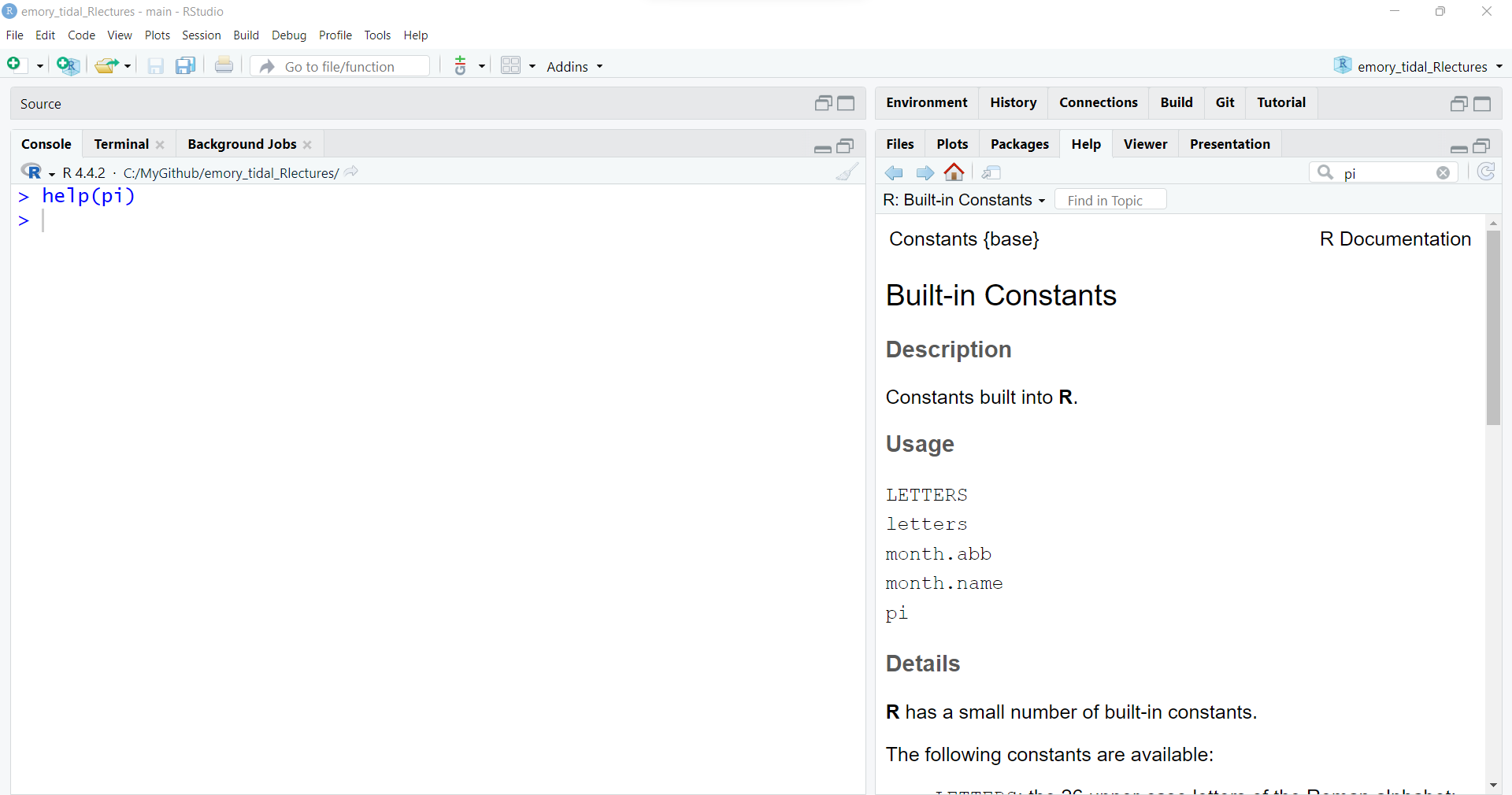
The help() function defaults to searching for a built-in object, function or dataset by default in the base R package. But some functions may exist in multiple packages, so it is always a good idea to add the package when running the help() function if possible.
Since pi is in the base R package, it would be better to run:
help(pi, package = "base")If you have no idea what package a function may be in, you can use the ?? search operator. For example, many packages include a plotting related function. If you want to see how many R packages currently installed on your computer have a plot related function, type the following:
??plotThe majority of the R programming language is driven by functions. Technically the + operator is actually a function that performs a sum.
You can even get help on these operators, by typing help("+"). We have to add the quotes "" so that R knows we are looking for this operator and not trying to perform an addition operation inside the function call.
help("+")But let’s try a function to create a sequence of numbers - for example, let’s use the seq() function to create a sequence of numbers from 1 to 10.
seq(10) [1] 1 2 3 4 5 6 7 8 9 10And let’s look at the help page for the seq() function.
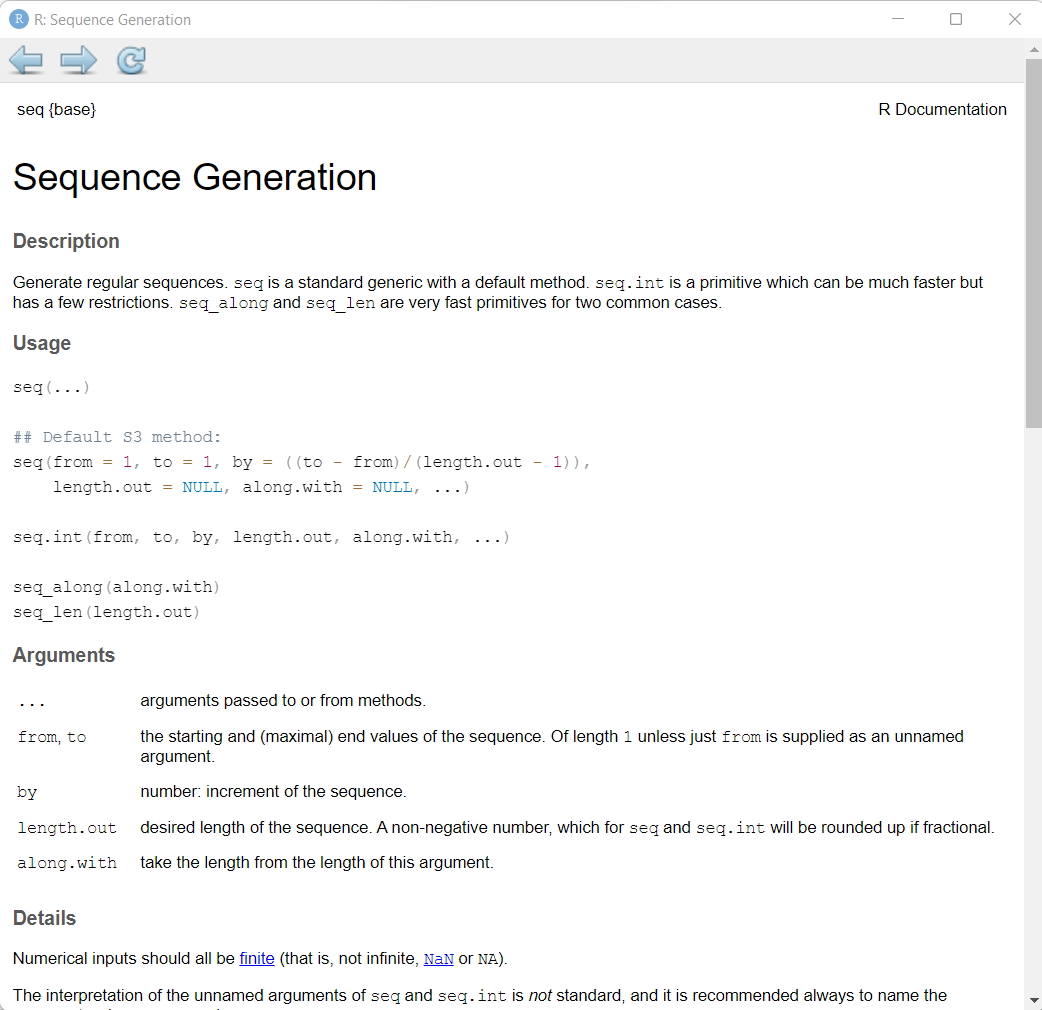
R allows for what is called “lazy” coding. This basically means you can provide very minimal input and R will try to figure out what you want using the default settings for a given function. In the case of seq() the function begins by default at 1 and creates the output in steps of 1 up to the value of 10.
While “lazy” coding practices are common with R, it would actually be better to explicitly define each argument to make sure you get the exact output you want. To do this, inside the parentheses () we should assign a value to each argument.
Notice in the “Help” page for seq() shown above that the first 3 arguments are: from, to and by. Each of these can be defined inside the () by using the syntax of the name of the argument, an equals sign =, and then the value (or object) you want to assign:
\[argument = value\]
For example, the explicit function call should be:
seq(from = 1,
    to = 10,
    by = 1)
[1] 1 2 3 4 5 6 7 8 9 10You could easily change these values to get a sequence from 0 to 5 in increments of 0.1 as follows:
seq(from = 0,
    to = 5,
    by = 0.1)
[1] 0.0 0.1 0.2 0.3 0.4 0.5 0.6 0.7 0.8 0.9 1.0 1.1 1.2 1.3 1.4 1.5 1.6 1.7 1.8
[20] 1.9 2.0 2.1 2.2 2.3 2.4 2.5 2.6 2.7 2.8 2.9 3.0 3.1 3.2 3.3 3.4 3.5 3.6 3.7
[39] 3.8 3.9 4.0 4.1 4.2 4.3 4.4 4.5 4.6 4.7 4.8 4.9 5.0Notice the incremental counter [#] on the left to help you keep track of how many elements are in the resulting numeric vector that was the “result” or “output” from the seq() function.
So, as you can tell, the R Console is useful but slow and tedious. Let’s create an R script to save all of these commands in a file so that we can easily access everything we’ve done so far and re-run these commands as needed.
It is a good coding practice to create R code (saved in *.R script files or *.Rmd Rmarkdown files) for every step in your data preparation and analysis so that:
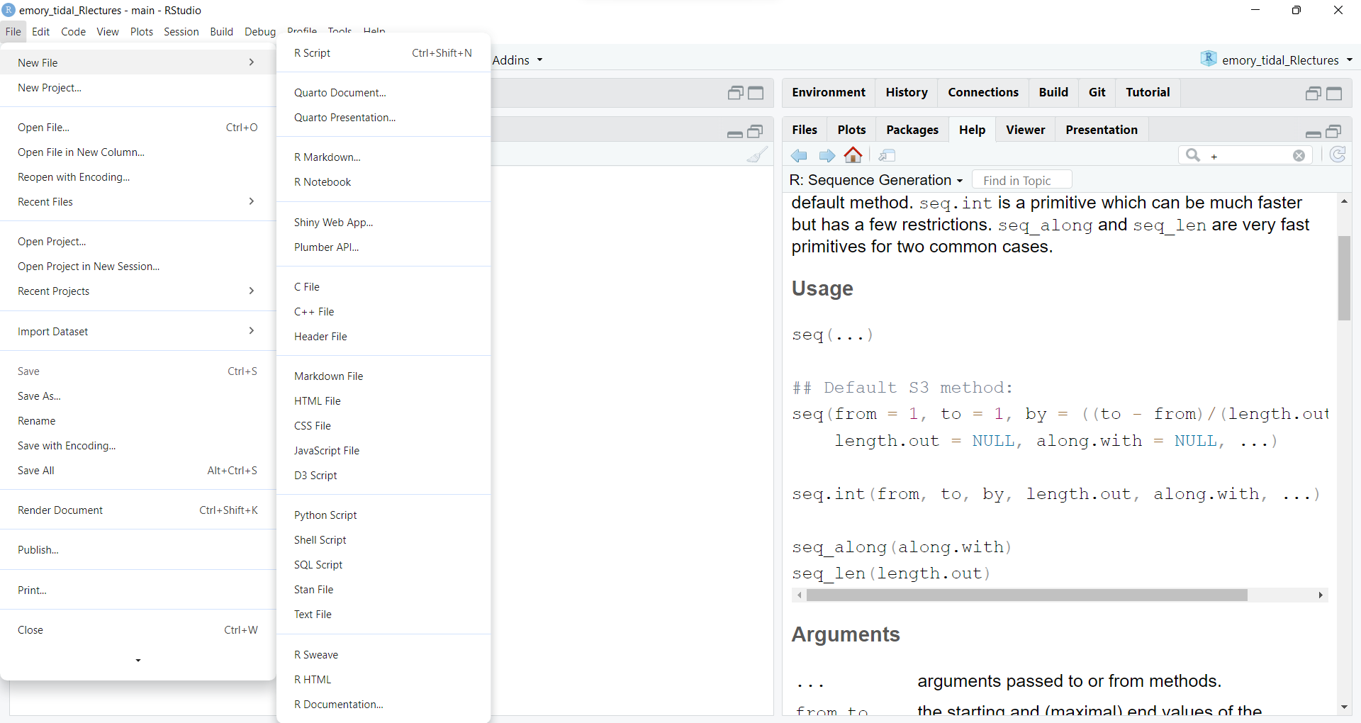
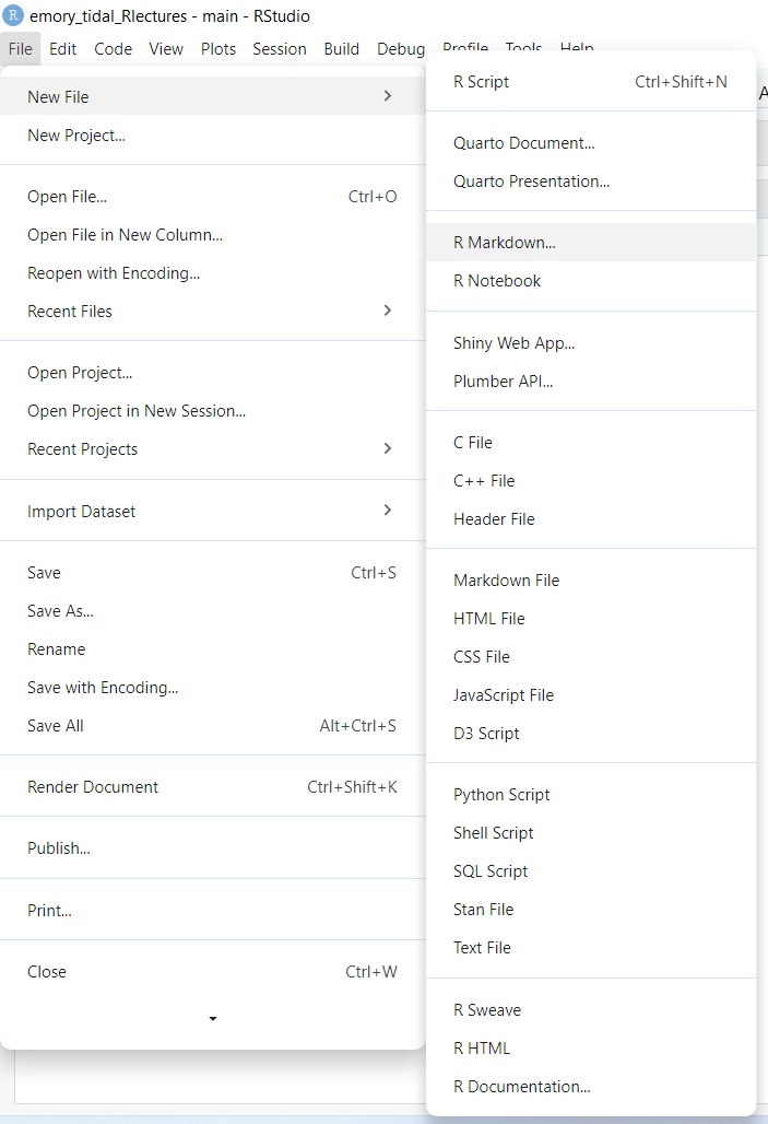
In RStudio go to the top menu “File/New File/R Script”:
Once the R Script file is created, type in some of the commands we did above in the Console and put one command on each line.
Just select each line and click “Run”.
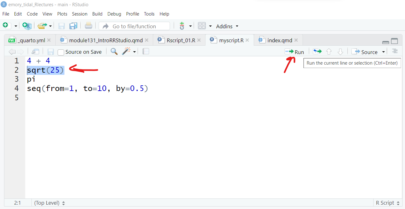
Then you can save the file on your computer as “myscript.R”, for example.
You can also select all of the rows and click run to execute all of the code in sequence and see the output in the “Console” Window.
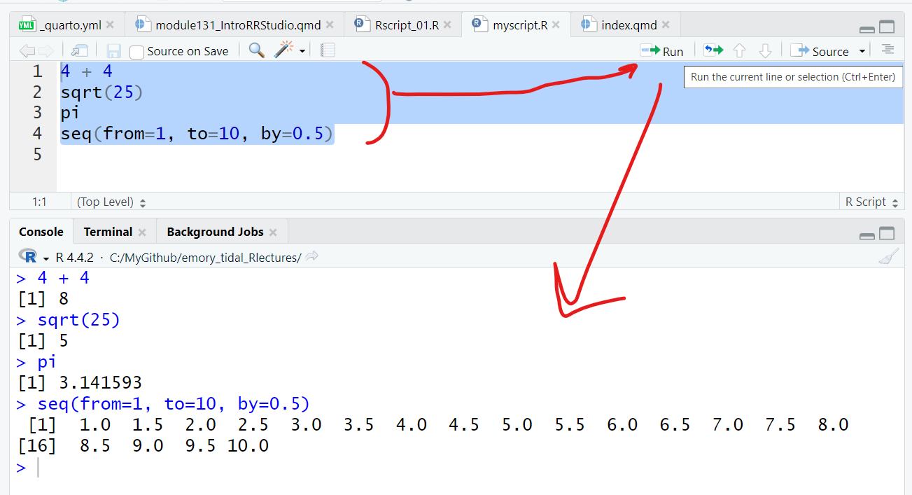
Here is the code and output:
4 + 4[1] 8sqrt(25)[1] 5pi[1] 3.141593seq(from=1, to=10, by=0.5) [1] 1.0 1.5 2.0 2.5 3.0 3.5 4.0 4.5 5.0 5.5 6.0 6.5 7.0 7.5 8.0
[16] 8.5 9.0 9.5 10.0Let’s try out some more built-in R functions, save the output in objects in your “Global Environment” and then use them in other functions and subsequent analysis steps.
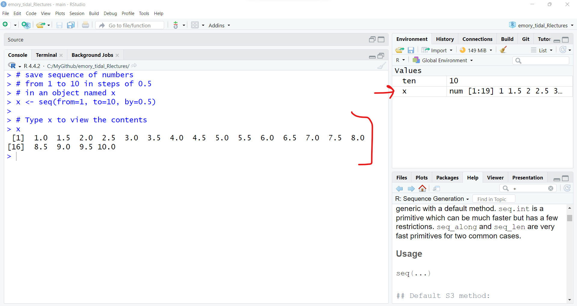
Create a sequence of numbers and save them as an object called x. I also added a comment in the R code block below. Everything after the # hashtag is a comment which R will ignore. It is a good idea to add comments in your code to make sure that you and others understand what each part of your code does (including yourself in a few weeks when you’ve forgotten why you wrote that code step).
# save sequence of numbers
# from 1 to 10 in steps of 0.5
# in an object named x
x <- seq(from=1, to=10, by=0.5)

# Type x to view the contents
x
[1] 1.0 1.5 2.0 2.5 3.0 3.5 4.0 4.5 5.0 5.5 6.0 6.5 7.0 7.5 8.0
[16] 8.5 9.0 9.5 10.0Also take a look at the “Global Environment” to see the new object x.
# use x to create new object y
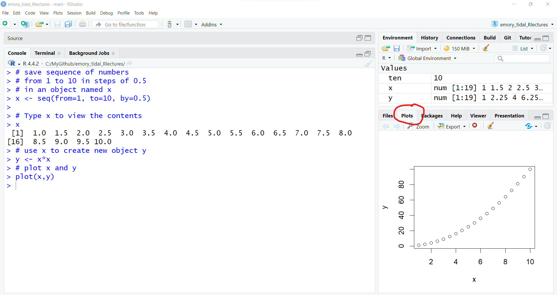
y <- x*xOnce the object y is created, we can make a simple 2-dimensional scatterplot using the built-in plot() base R function.
# plot x and y
plot(x,y)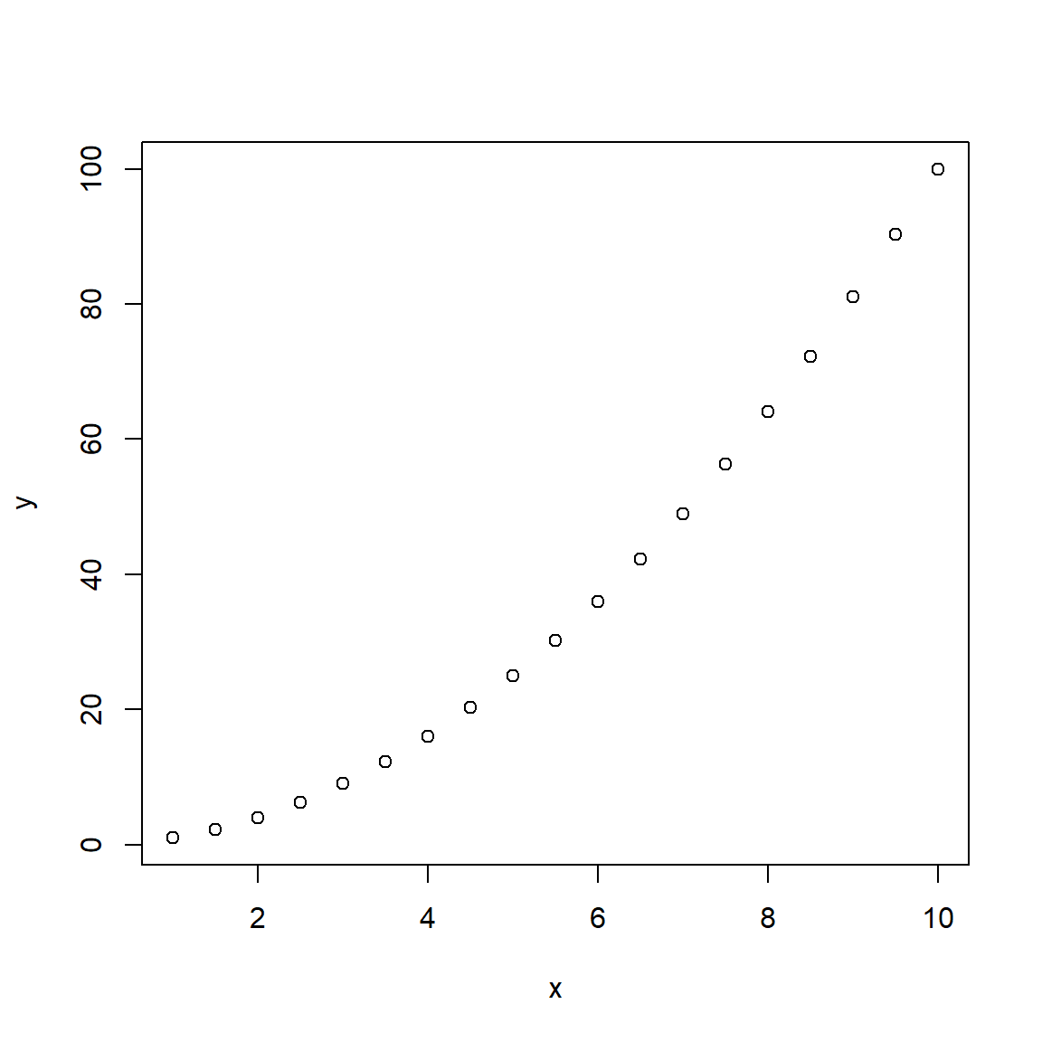
The plot is shown above, but if you are running this code interactively in the RStudio desktop, check the “Plots” window pane (lower right).
Download Rscript_01.R (right click the linked file and “Save As” the file on your computer), then open it in your RStudio and run through the code. Try out new variations on your own.
sessionInfo()
While the base installation of R is pretty powerful on it’s own, the beauty of R and the R programming community is that there are literally hundreds of thousands if not millions of people programming in R and creating new functions everyday.
In order to use these new functions, the developers put them together in packages that we can install to extend the functionality of R.
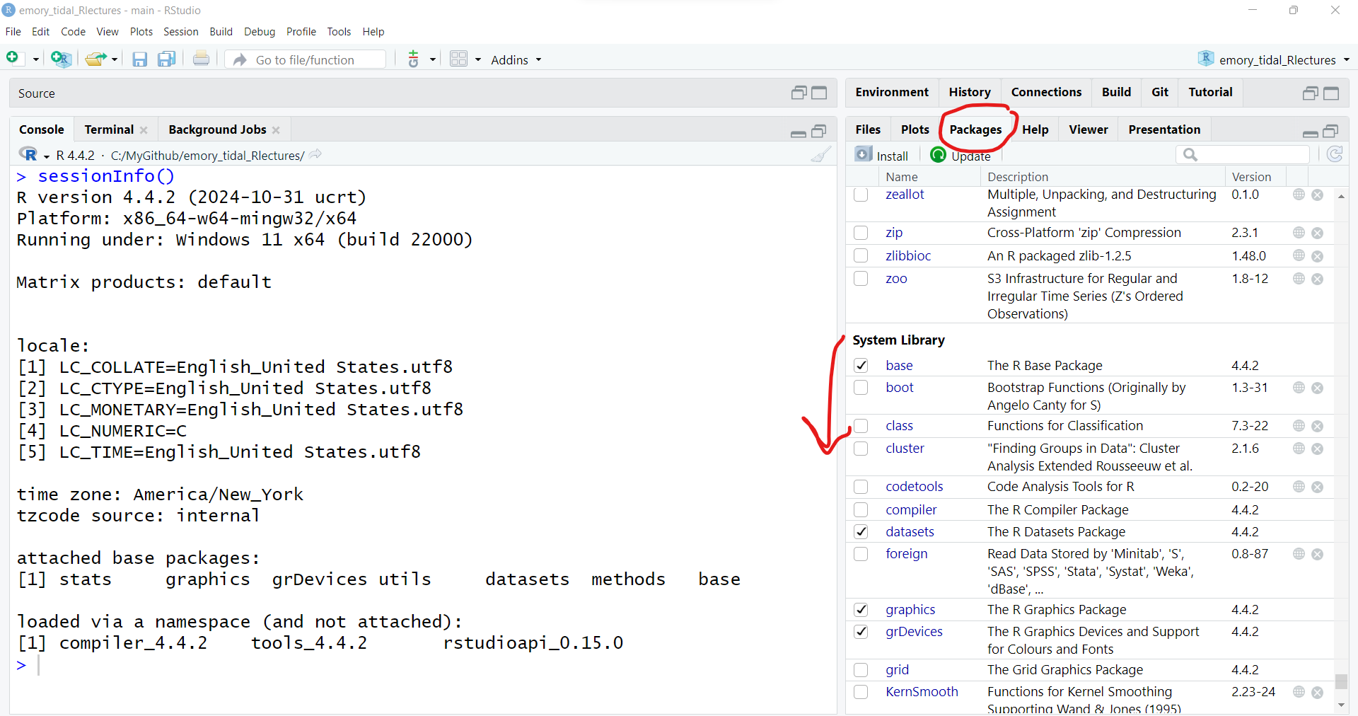
But first, let’s take a look at the packages that are part of the basic installation of R. One way to see which packages are currently installed and loaded into your current R computing session, is by running the command sessionInfo().
Notice: This function name is all lowercase except for the capital “I” in the middle. Be sure you are typing sessionInfo() and not sessioninfo().
You will also notice that the sessionInfo() command also lists the version of R I’m currently running (4.4.2), my operating system (Windows 11) and and my locale (USA, East Coast). These details can sometimes be helpful for collaborating with others who may be working with different system settings and for debugging errors.

The basic installation of R includes 7 packages:
statsgraphicsgrDevicesutilsdatasetsmethodsbaseTo learn more click on the “Packages” TAB in the lower right window pane to see the list of packages installed on your computer. I have a lot of packages on my computer, but here is a screenshot of the base R packages.
See the packages listed under “System Library” which are the ones that were installed with base R. You’ll notice that only some of these have checkmarks next to them. The checkmark means those are also loaded into your R session. Only some of them are loaded into memory by default to minimize the use of your computer’s memory.
Let’s install a “new” R package, like ggplot2.
Go to the RStudio menu “Tools/Install” Packages
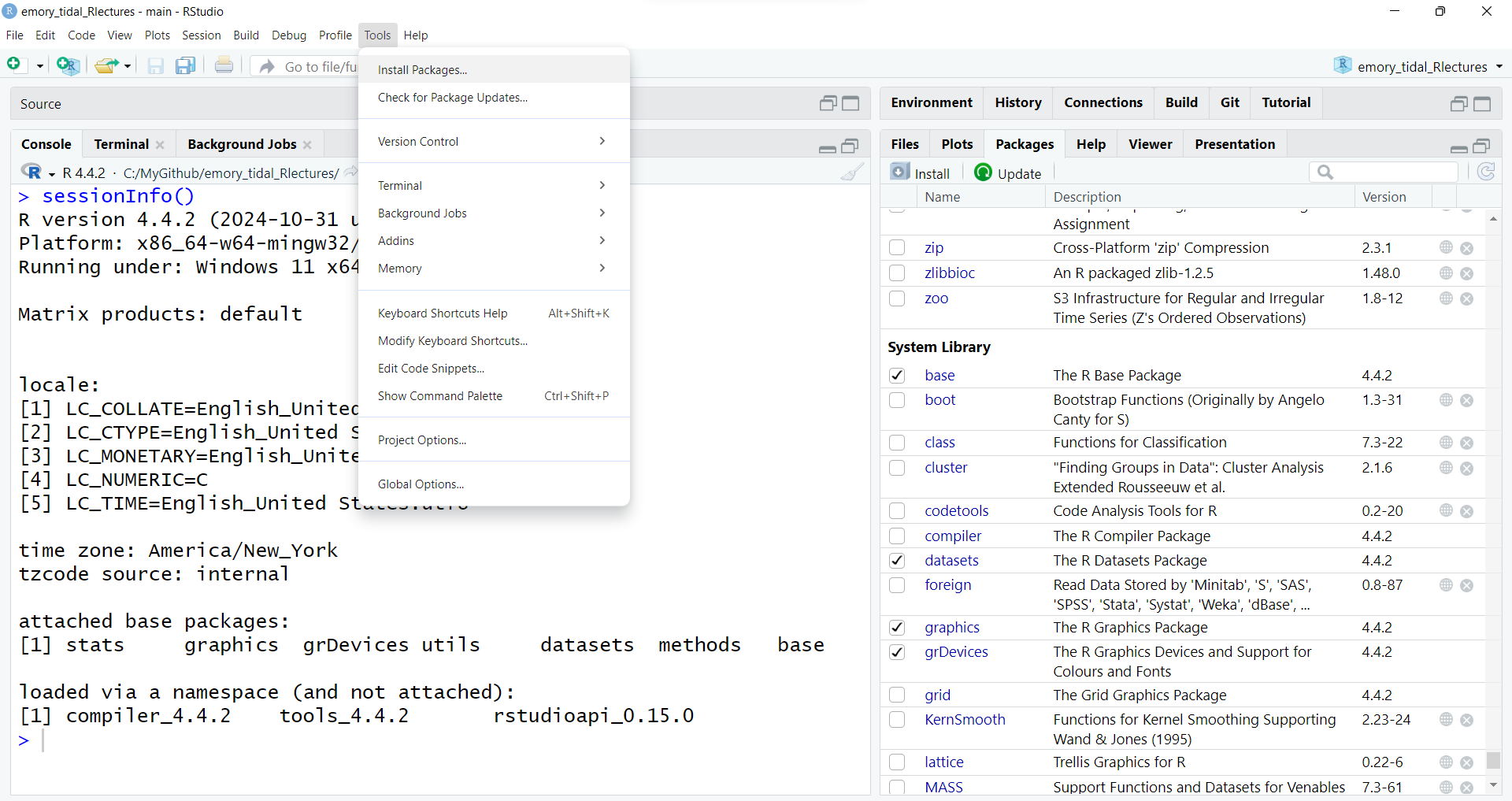
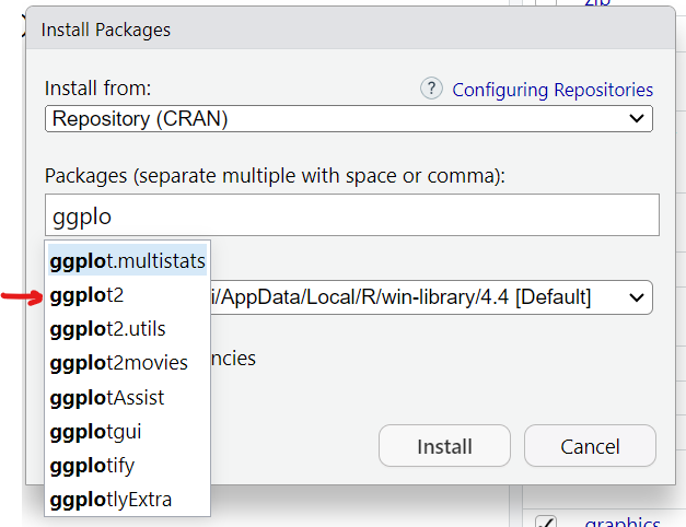
This will then open up a window where you can type in the name of the package you want. As soon as we start typing ggplot2 the menu begins listing all packages with that partial spelling…
You’ll notice that there are 3 parts to the installation:
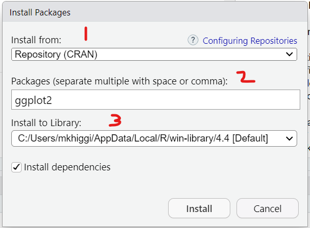
Using the “Tools/Install” Packages menu from within RStudio automatically links to CRAN, which is the “The Comprehensive R Archive Network”. You’ve already been here once to download and install the R programming language application.
Here is a screenshot of the CRAN homepage.
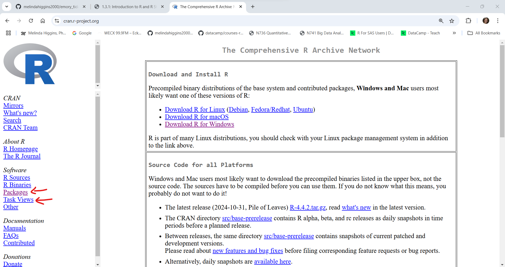
Next click on “Packages” at the left to see the full list of packages currently available. As of right now (01/10/2025 at 5:12pm EST) there are 21,872 packages. This number increases every day as people create, validate and publish their packages on CRAN. You can get a list of all of the packages or if you have no idea what package you need, you can also look at the “Task Views” to see groupings of packages.
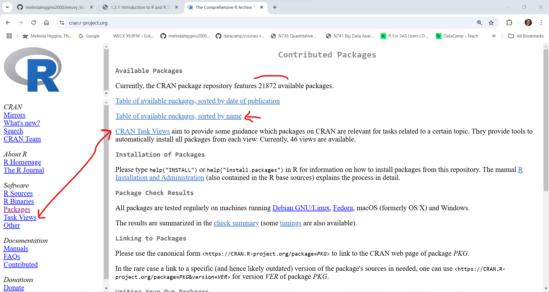
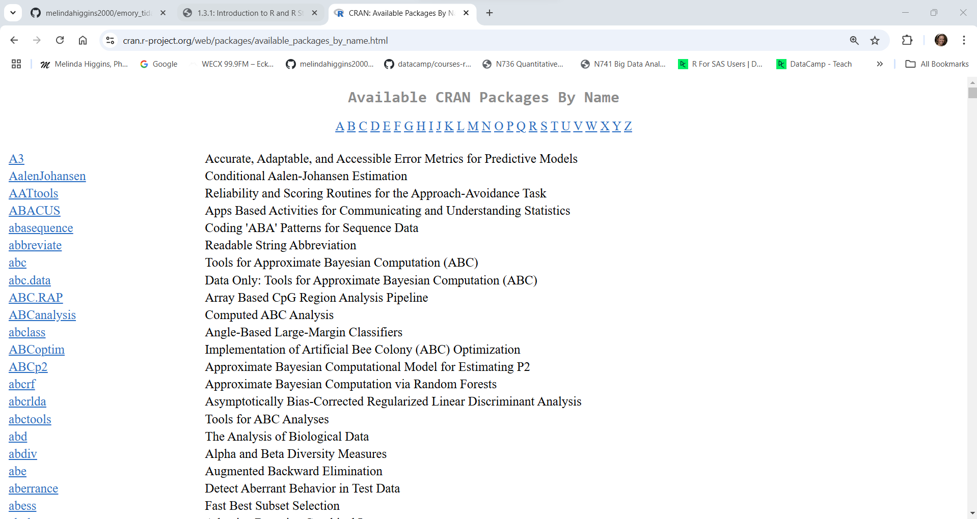
Here is what the list of Packages looks like sorted by name:
However, you can also browse Packages by “Task View”:
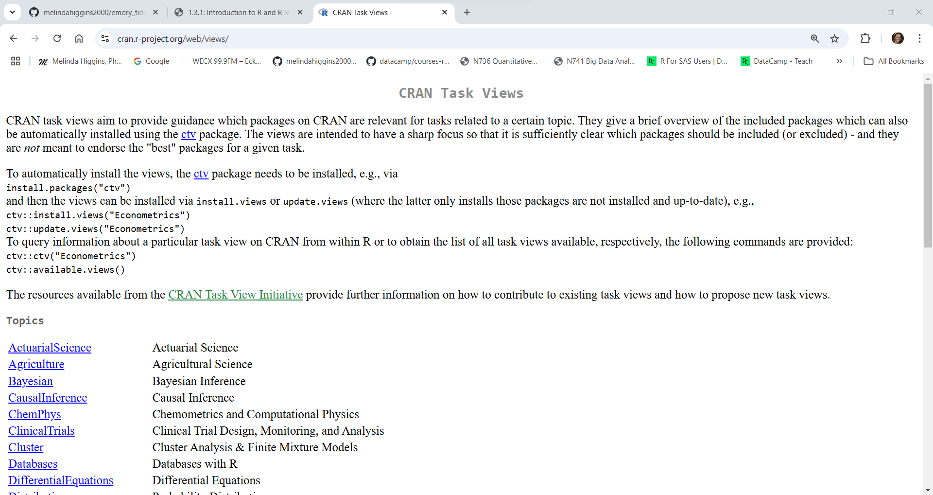
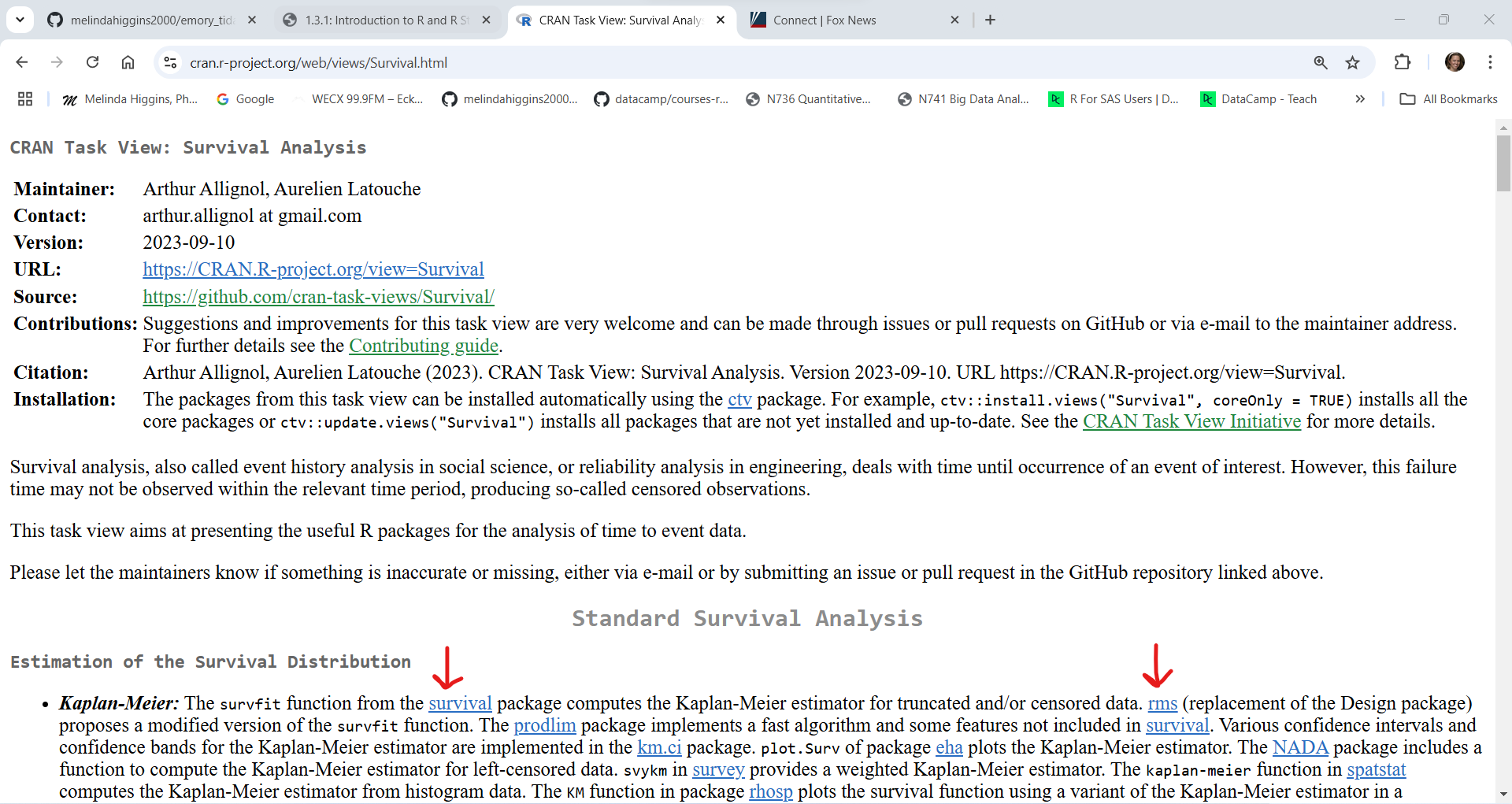
For example, suppose you are interested in survival analysis, here is a screenshot of the Survival Task View.
As you can see each Task View has a person(s) listed who help to maintain these collections. As you scroll through the webpage, you’ll see links to packages they recommend along with a description of what the packages do. For example, see the links below to the survival and rms packages.
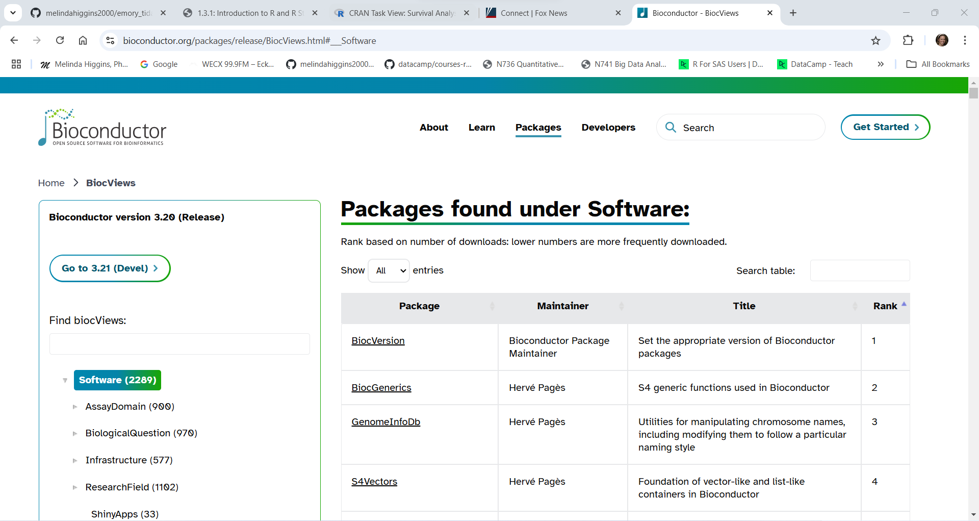
While the list of R packages on CRAN is impressive, if you plan to do analyses of biological data, there is a good chance you will need a package from Bioconductor.org.
As of right now (01/10/2025 at 6:45pm EST) there are 2289 packages on Bioconductor. Similar to CRAN, Bioconductor requires each package to meet certain validation criteria and code testing requirements but these criteria are even more stringent on Bioconductor than on CRAN. You’ll notice that you can search for packages under the biocViews (left side column) or you can sort them alphabetically or search for individual packages in the section on the right side.
The one disadvantage of R packages from Bioconductor is that you cannot install them directly using the RStudio menu for “Tools/Install” Packages because you cannot “see” the Bioconductor repository from inside RStudio. Instead you have to install Bioconductor packages using R code.
For example, here is what you need to do to install the phyloseq package which “… provides a set of classes and tools to facilitate the import, storage, analysis, and graphical display of microbiome census data”.
To install phyloseq you need to (see the black box of code in the screenshot shown below):
BiocManager from CRAN - this package you can install from the RStudio menu for “Tools/Install Packages” - or you can run the code shown below for install.packages().install.packages("BiocManager")BiocManager::install("phyloseq")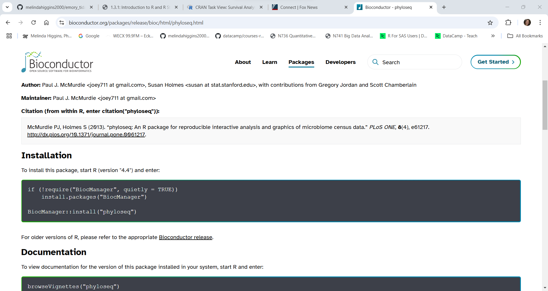
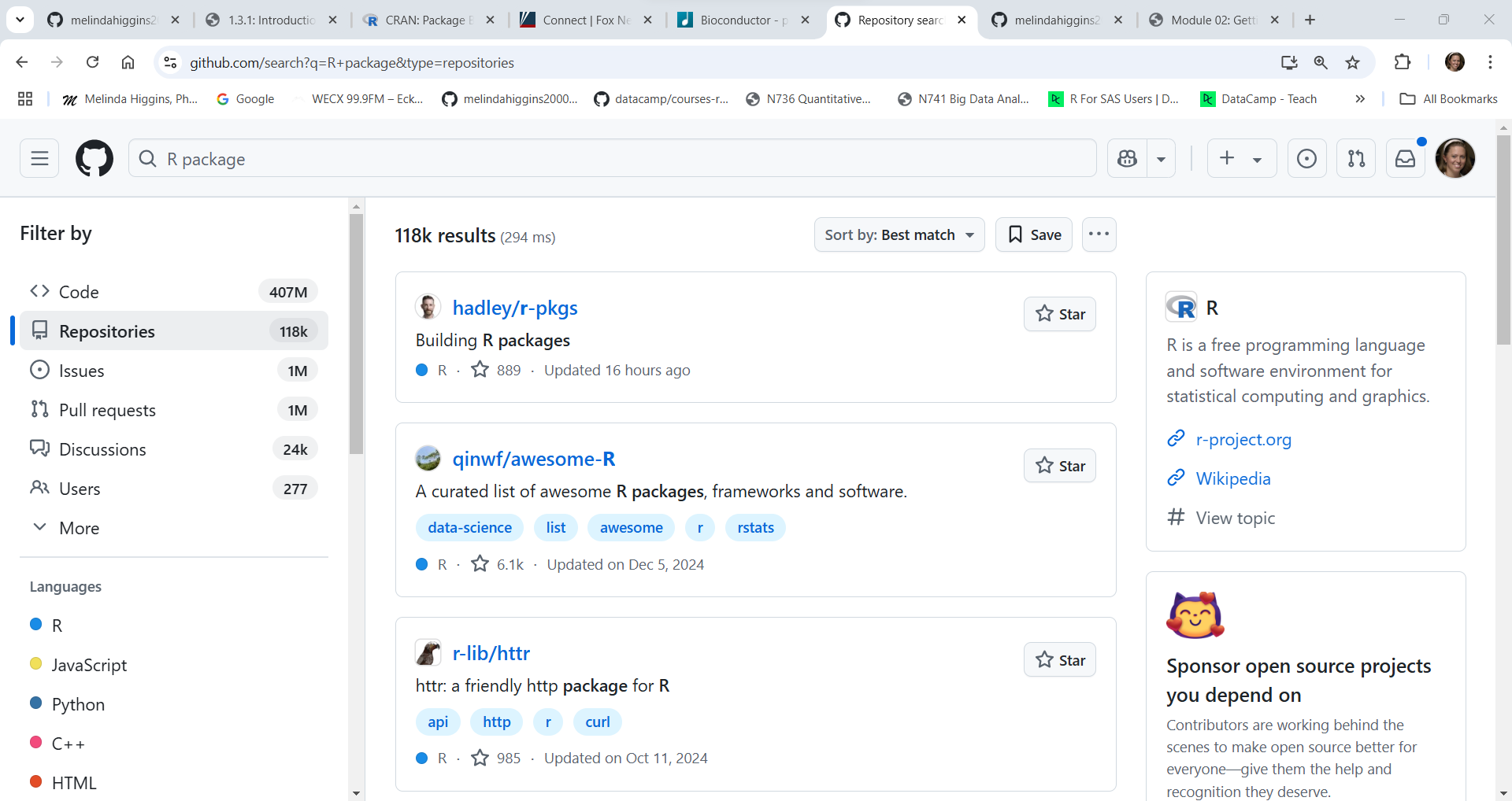
In addition to the CRAN and Bioconductor repositories, you can also get packages from Github (and other cloud-based repositories), friends, teammates or write your own.
To get an idea of how many packages may be currently on Github, we can “search” for “R package” at https://github.com/search?q=R+package&type=repositories and as you can see this is well over 118,000+ packages.
While you can find packages on Github that have not (yet) been published on CRAN or Bioconductor, the developers of packages currently on CRAN and Bioconductor also often publish their development version (think of these as in “beta” and still undergoing testing) on Github.
For example, the current published version of the data wrangling R package dplyr on CRAN was last updated on 11/17/2023 (over a year ago).
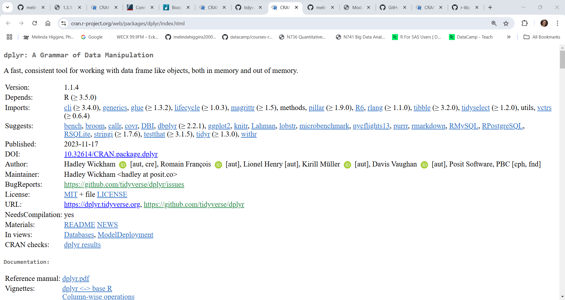
However, the development version of dplyr on Github was last updated 5 months ago in August 2024. So, there is probably a new version of dplyr coming soon for CRAN.
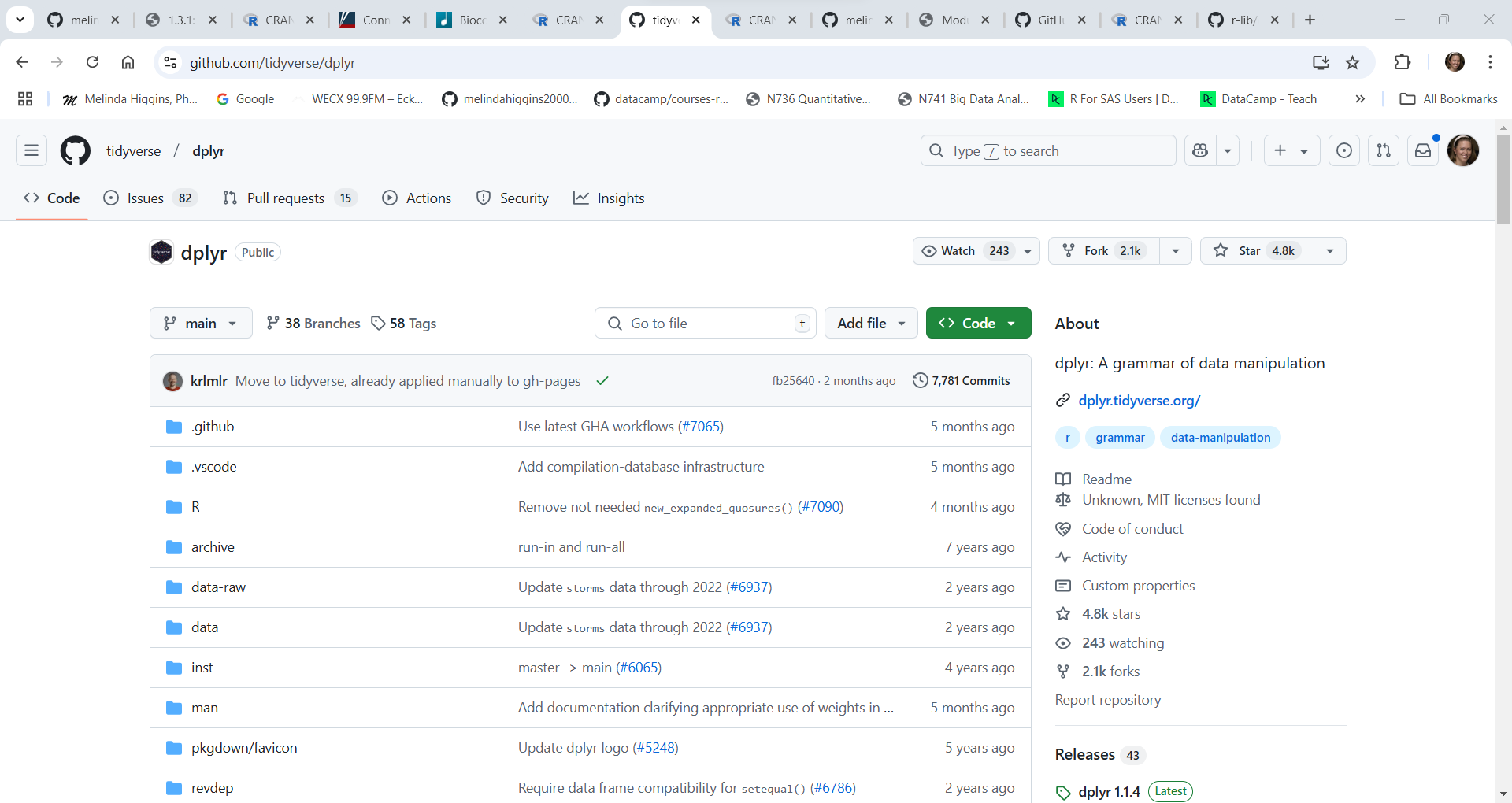
While the developers haven’t published this “Github” version of dplyr yet on CRAN, if you want to test out new dplyr functions and updates under development, you can go to the R Console or write an R script to install the development version using these commands (see below) which is explained on the dplyr on Github website.
# install.packages("pak")
pak::pak("tidyverse/dplyr")So, as you have seen there are numerous ways to find R packages and there are hundreds of thousands of them out there. Your company or team may also have their own custom R package tailored for your specific research areas and data analysis workflows.
Finding R packages is similar to finding new questionnaires, surveys or instruments for your research. For example, if you want to measure someone’s depression levels, you should use a validated instrument like the Center for Epidemiological Studies-Depression (CESD) or the Beck Depression Index (BDI). These measurement instruments have both been well published and are well established for depression research.
Finding R packages is similar - do your research! Make sure that the R package has been published and is well established to do the analysis you want. In terms of reliability, getting packages from CRAN or Bioconductor are the best followed by Github or other individuals. The best suggestion is look to see which R packages are being used by other people in your field.
While it may seem worrisome that there is no governing company or organization that verifies and validates and certifies all R packages, the good news is that the R community is a vast Global community. The development of R is not controlled by a limited number of people hired within a single company - instead there are literally millions of R programmers across the Globe testing and providing feedback on a 24/7 basis. If there is a problem with a package or function, there will be people posting about these issues - see Additional Resources.
This is the power of Open Source computing!!
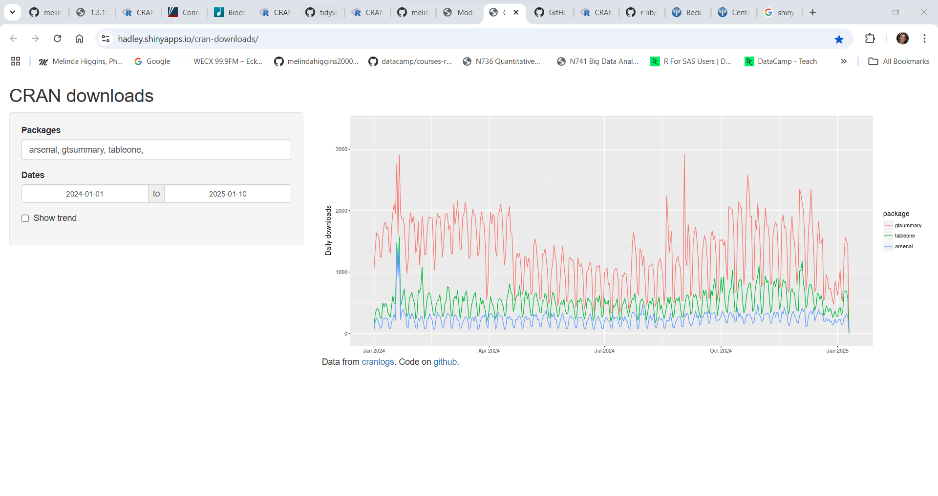
To get an idea of how long a package has been in use and if it is still being actively supported and how it relates to other similar packages, check out this interactive Shiny app website for package downloads from CRAN https://hadley.shinyapps.io/cran-downloads/. Type in the packages you want (separated by commas) to compare and put in the date range of interest.
Here is an example comparing the arsenal, gtsummary, and tableone packages all of which are useful for making tables of summary statistics (aka, “Table 1”) - showing the number of downloads since the beginning of Jan 1, 2024.
As you can see the most downloaded of these 3 packages is gtsummary followed by tableone and then arsenal having the fewest downloads. This does NOT necessarily imply quality, but it does give you some insight into the popularity of these packages. I actually prefer the arsenal table package but tableone has been around longer and gtsummary is written by members of the RStudio/Posit development community and is more well known and popular. All 3 of these packages can be found in use in current research literature.
You will see examples of all 3 of these table-making packages in Module lesson 1.3.2
Here is an example of two specific packages I like. The rggobi package which was great for visualizing multiple dimensions of data simultaneously but which is no longer supported. But there is now a newer tourr package which was written by the same developers to replace the rggobi package. You can see that in the middle of 2020, the number of downloads for rggobi dropped almost to 0 and the tourr package downloads started to rise - this is about when rggobi was archived on CRAN and they switched over to maintaining the newer tourr package.
rggobi on CRAN moved to archived status in July 2020, buttourr on CRAN was last updated in April 2024.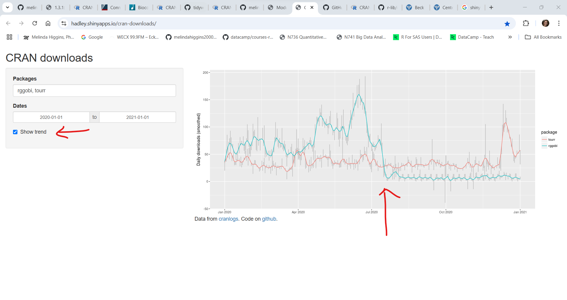
In summary:
After you’ve decided what package you want and have installed it onto your computer, you must load it into memory for EVERY new R session for which you want those functions available.
Unless you upgrade R or change computers, you only need to install a given R package once. But you do need to (re)-load the package into your current R session every time you (re)-start R (or RStudio).
For example, suppose I want to make a plot using the ggplot2 package. Before I can use the ggplot() function, I have to load that package into my computing session.
Here is my current R session status BEFORE I load the ggplot2 package.
# show current sessionInfo
sessionInfo()
R version 4.6.0 (2026-04-24 ucrt)
Platform: x86_64-w64-mingw32/x64
Running under: Windows 11 x64 (build 22000)
Matrix products: default
LAPACK version 3.12.1
locale:
[1] LC_COLLATE=English_United States.utf8
[2] LC_CTYPE=English_United States.utf8
[3] LC_MONETARY=English_United States.utf8
[4] LC_NUMERIC=C
[5] LC_TIME=English_United States.utf8
time zone: America/New_York
tzcode source: internal
attached base packages:
[1] stats graphics grDevices utils datasets methods base
loaded via a namespace (and not attached):
[1] htmlwidgets_1.6.4 compiler_4.6.0 fastmap_1.2.0 cli_3.6.5
[5] tools_4.6.0 htmltools_0.5.9 rstudioapi_0.17.1 yaml_2.3.10
[9] rmarkdown_2.31 knitr_1.51 jsonlite_2.0.0 xfun_0.53
[13] digest_0.6.39 rlang_1.2.0 evaluate_1.0.5 Since I have not yet loaded the ggplot2 package into the session, I will get an error.
# I have not yet loaded ggplot2 into the session
# try the ggplot() function with the
# built-in pressure dataset to see error
ggplot(pressure, aes(temperature, pressure)) +
  geom_point()
Error in `ggplot()`:
! could not find function "ggplot"The code above generates an error since these functions are not yet available in our session.
To fix this error, we need to use the library() function to load the ggplot2 functions into current working memory.
# load ggplot2 package
library(ggplot2)

# look at sessionInfo again
sessionInfo()
R version 4.6.0 (2026-04-24 ucrt)
Platform: x86_64-w64-mingw32/x64
Running under: Windows 11 x64 (build 22000)
Matrix products: default
LAPACK version 3.12.1
locale:
[1] LC_COLLATE=English_United States.utf8
[2] LC_CTYPE=English_United States.utf8
[3] LC_MONETARY=English_United States.utf8
[4] LC_NUMERIC=C
[5] LC_TIME=English_United States.utf8
time zone: America/New_York
tzcode source: internal
attached base packages:
[1] stats graphics grDevices utils datasets methods base
other attached packages:
[1] ggplot2_4.0.1
loaded via a namespace (and not attached):
[1] vctrs_0.7.3 cli_3.6.5 knitr_1.51 rlang_1.2.0
[5] xfun_0.53 generics_0.1.4 S7_0.2.0 jsonlite_2.0.0
[9] glue_1.8.0 htmltools_0.5.9 scales_1.4.0 rmarkdown_2.31
[13] grid_4.6.0 evaluate_1.0.5 tibble_3.3.0 fastmap_1.2.0
[17] yaml_2.3.10 lifecycle_1.0.5 compiler_4.6.0 dplyr_1.2.1
[21] RColorBrewer_1.1-3 pkgconfig_2.0.3 htmlwidgets_1.6.4 rstudioapi_0.17.1
[25] farver_2.1.2 digest_0.6.39 R6_2.6.1 tidyselect_1.2.1
[29] pillar_1.11.0 magrittr_2.0.4 withr_3.0.2 tools_4.6.0
[33] gtable_0.3.6 Notice that under other attached packages we can now see ggplot2_3.5.1 indicating that yes ggplot2 is installed and in memory and that version 3.5.1 is the version I am currently using.
Let’s try the plot again with the ggplot() function from the ggplot2 package.
# try the plot again
ggplot(pressure, aes(temperature, pressure)) +
  geom_point()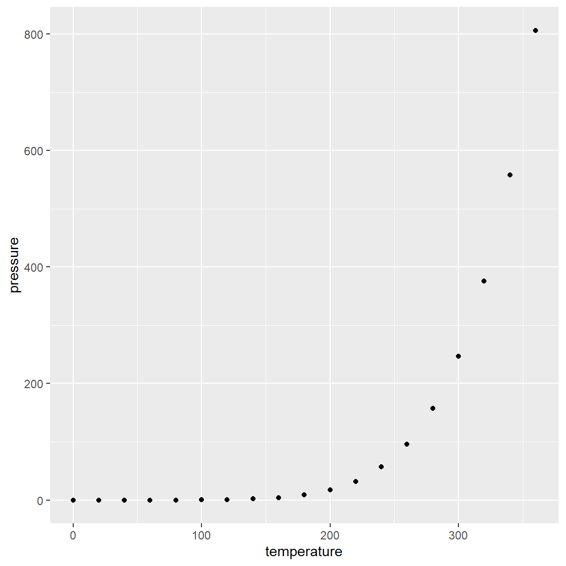
Everything you close out your R/RStudio computing session (or restart your R session) you will need to load all of your package again. I know this seems like a HUGE pain, but there is a rationale for this.
library() function.BUT … If you do have a core set of packages that you would like to make sure get loaded into memory every time you start R/RStudio, see these helpful posts on customizing your startup:
We will do more in the later lesson 1.3.6: Putting reproducible research principles into practice, but let’s take a look at an Rmarkdown file and how we can use it to create a report that combines together data + code + documentation to produce a seamless report.
Go to the RStudio menu and click “File/New File/R Markdown”:
Type in a title, your name, the date and choose the format you’d like to create. For your first document I encourage you to try HTML. But you can create WORD (DOC) documents and even PDFs. In addition to documents, you can also create slide deck presentations, Shiny apps and other custom products like R packages, websites, books, dashboards and many more.
To get started, use the built-in template:
*.html file.
tinytex https://yihui.org/tinytex/ R package to create PDFs.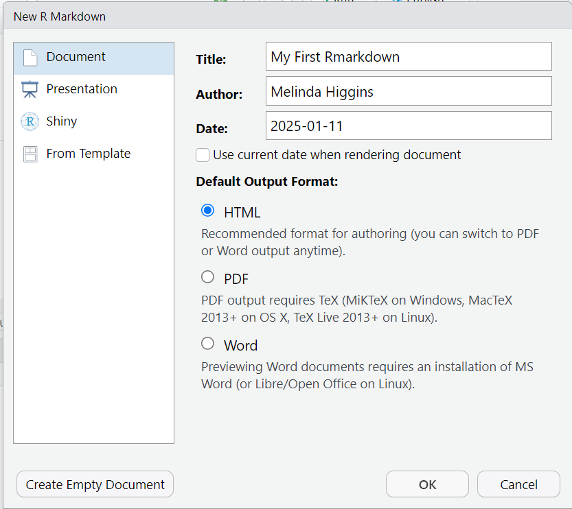
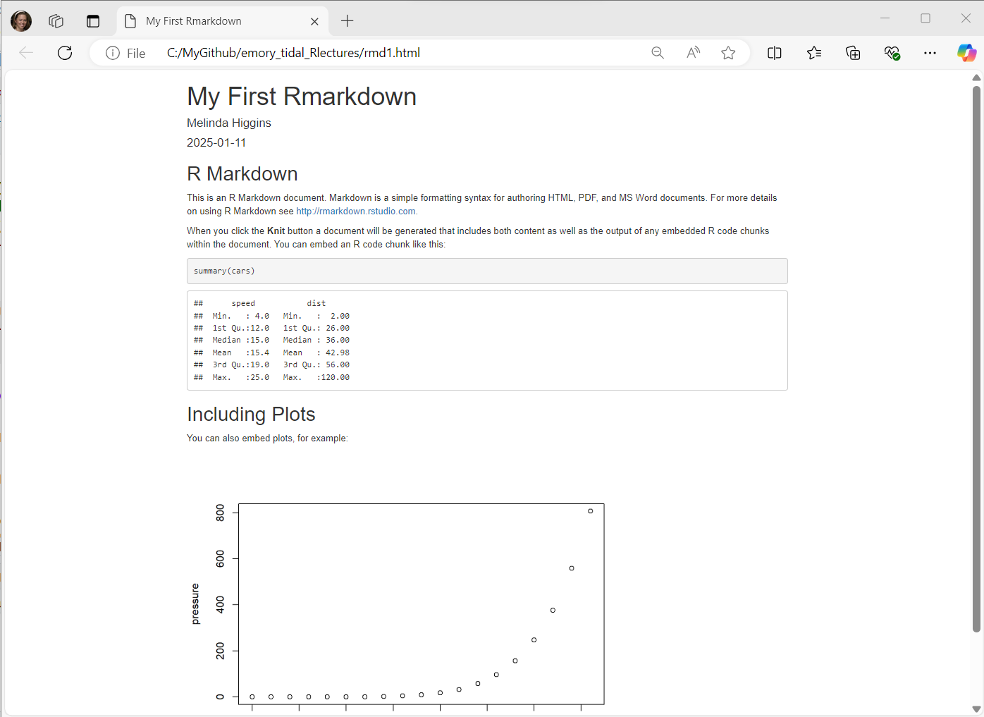
Here is the Example RMarkdown Template provided by RStudio to help you get started with your first Rmarkdown document.
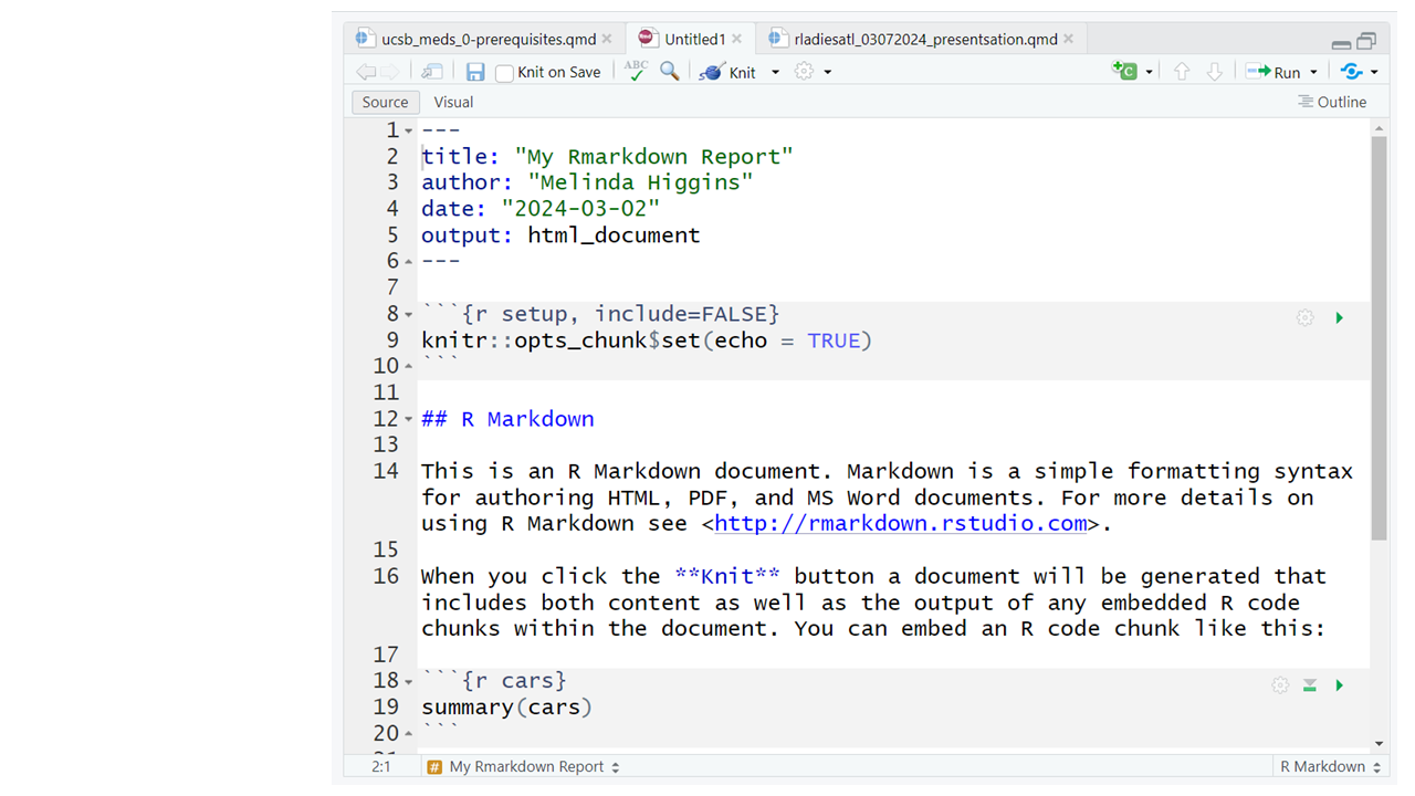
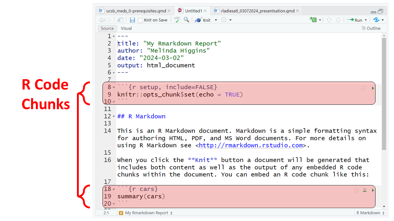
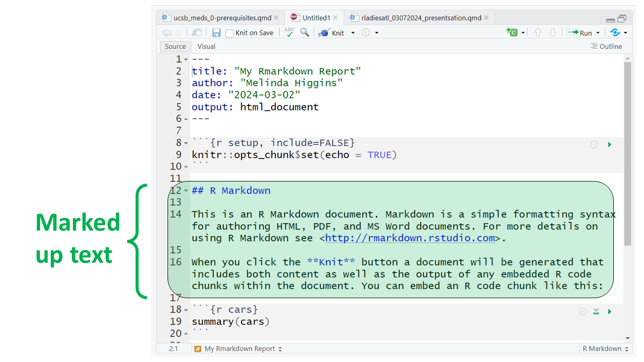
This document consists of the following 3 key sections:
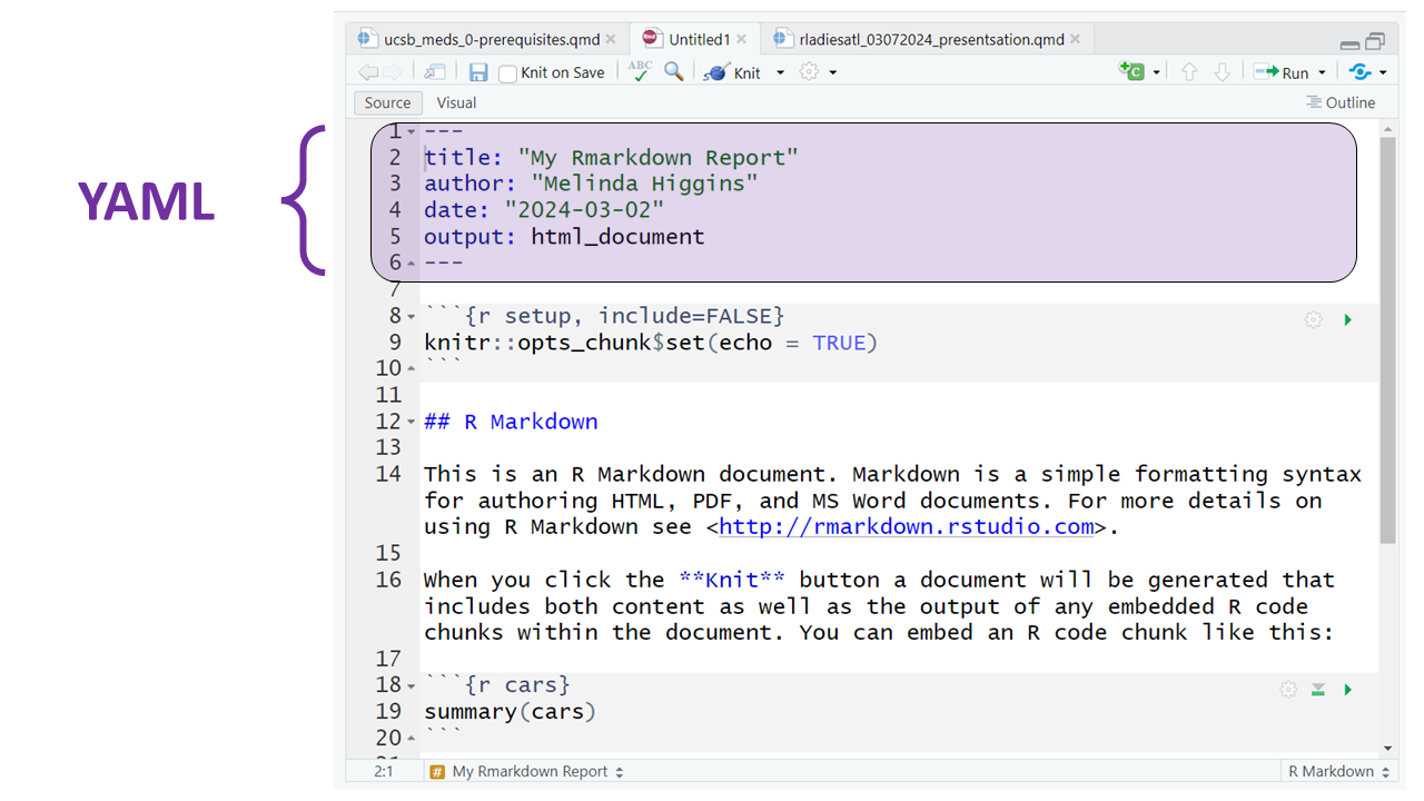
Notice that the code block starts and ends with 3 backticks ``` and includes the {r} Rlanguage designation inside the curly braces.
Rmarkdown can be used for many different programming languages including python, sas, and more, see rmarkdown - language-engines.
For example putting 2 asterisks ** before and after a word will make it bold, putting one _ underscore before and after a word will make the word italics; one or more hashtags # indicate a header at certain levels, e.g. 2 hashtags ## indicate a header level 2.
I encourage you to go through the step by step tutorial at https://rmarkdown.rstudio.com/lesson-1.html.
Here are all 3 sections outlined.
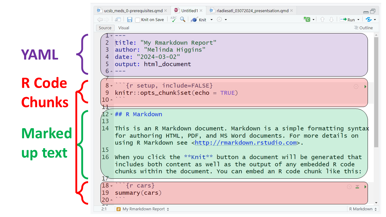
At the top of the page you’ll notice a little blue button that says “knit” - this will “knit” (or combine) the output from the R code chunks and format the text as “marked up” and produce this HTML file (which will open in a browser window):