1.3.5: Statistical Tests and Models

(In Person)

Session Objectives (updated)

  1. Develop linear regression models and explore results.
  2. Develop logistic regression models and explore results.
  3. Perform t-tests and ANOVA and explore results.
  4. Modeling with Complex Survey Weights

0. Prework - Before You Begin

A. Install packages

If you do not have them already, install the following packages from CRAN (using the RStudio Menu “Tools/Install” Packages interface):

B. Open/create an RStudio project for this lesson

Let’s start with the myfirstRproject RStudio project you created in Module 1.3.2 - part 1. If you have not yet created this myfirstRproject RStudio project, go ahead and create a new RStudio Project for this lesson. Feel free to name your project whatever you want, it does not need to be named myfirstRproject.


1. Develop linear regression models and explore results.

Linear Regression Modeling

As we saw briefly in Module 1.3.4 - section 2 on missing data in regression models, linear regression can be accomplished using the built-in lm() function.

lm() stands for linear models. You can use this function for building both regression and ANOVA (analysis of variance) type models. aov() is another option for ANOVA as well.

Let’s take a closer look at the little linear model we ran for the sleep dataset from the VIM package. We will run the regression model again and save the output to an object called lm1. Look at default output.

Using the lm() function and exploring output

# load VIM Package to get sleep dataset
library(VIM)

# run model for predicting "Sleep" from "Dream"
# save the output in lm1
lm1 <- lm(Sleep ~ Dream, data = sleep)

# look at default output
lm1

Call:
lm(formula = Sleep ~ Dream, data = sleep)

Coefficients:
(Intercept)        Dream  
      6.027        2.305  

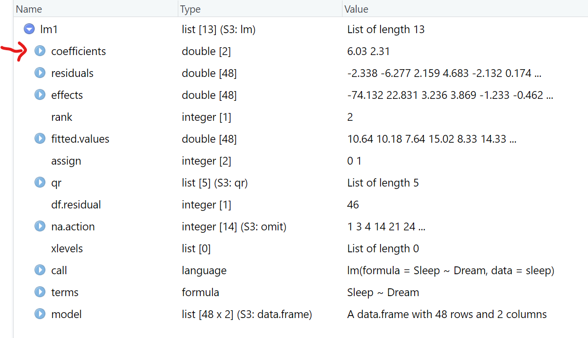
Let’s take a moment to take a look at the lm1 object in the Global Environment. Notice that only the intercept and slope terms are printed in the default output, but the lm1 object is actually a list of 13 elements only one of which are the “coefficients” from the model.

Next, to get more detailed output we need to run summary(lm1) which technically runs summary.lm() which is a special summary function specific for lm class type objects.

So, let’s save the summary(lm1) output and also take a look at that object slm1.

# save the summary of lm1
slm1 <- summary(lm1)

# look at default output
slm1

Call:
lm(formula = Sleep ~ Dream, data = sleep)

Residuals:
    Min      1Q  Median      3Q     Max 
-6.2765 -2.0384 -0.1096  2.1599  9.2624 

Coefficients:
            Estimate Std. Error t value Pr(>|t|)    
(Intercept)   6.0273     0.7960   7.572 1.27e-09 ***
Dream         2.3051     0.3209   7.183 4.85e-09 ***
---
Signif. codes:  0 '***' 0.001 '**' 0.01 '*' 0.05 '.' 0.1 ' ' 1

Residual standard error: 3.178 on 46 degrees of freedom
  (14 observations deleted due to missingness)
Multiple R-squared:  0.5287,    Adjusted R-squared:  0.5184 
F-statistic: 51.59 on 1 and 46 DF,  p-value: 4.849e-09

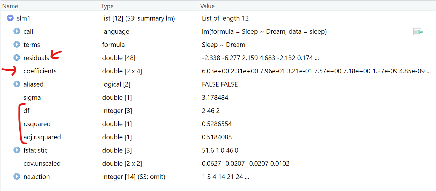
But here is what is in the slm1 object in the Global Environment - also a list with 12 elements. We get the coefficients again, but we get even more info - including the df (degrees of freedom), r.squared and adj.r.squared.

Nicer formatted regression table using gtsummary::tbl_regression

We can get a nicer output using the gtsummary::tbl_regression() table.

Characteristic Beta 95% CI1 p-value
Dream 2.3 1.7, 3.0 <0.001
1 CI = Confidence Interval

More output options for regression using easystats

Another suite of R packages that can be helpful to explore is the easystats package suite. In this example we will look at:

  • model_parameters() from the parameters package that is part of easystats package suite; and
  • report() from the report package that is also part of the easystats package suite.

Better formatted output table:

library(easystats)
model_parameters(lm1)
Parameter   | Coefficient |   SE |       95% CI | t(46) |      p
----------------------------------------------------------------
(Intercept) |        6.03 | 0.80 | [4.43, 7.63] |  7.57 | < .001
Dream       |        2.31 | 0.32 | [1.66, 2.95] |  7.18 | < .001

A nice summary with suggested interpretation verbiage:

report(lm1)
We fitted a linear model (estimated using OLS) to predict Sleep with Dream
(formula: Sleep ~ Dream). The model explains a statistically significant and
substantial proportion of variance (R2 = 0.53, F(1, 46) = 51.59, p < .001, adj.
R2 = 0.52). The model's intercept, corresponding to Dream = 0, is at 6.03 (95%
CI [4.43, 7.63], t(46) = 7.57, p < .001). Within this model:

  - The effect of Dream is statistically significant and positive (beta = 2.31,
95% CI [1.66, 2.95], t(46) = 7.18, p < .001; Std. beta = 0.73, 95% CI [0.52,
0.93])

Standardized parameters were obtained by fitting the model on a standardized
version of the dataset. 95% Confidence Intervals (CIs) and p-values were
computed using a Wald t-distribution approximation.

Other options within tidyverse packages

In the broom package there are some additional functions that are helpful for exploring the model fit metrics and more.

# A tibble: 2 × 5
  term        estimate std.error statistic       p.value
  <chr>          <dbl>     <dbl>     <dbl>         <dbl>
1 (Intercept)     6.03     0.796      7.57 0.00000000127
2 Dream           2.31     0.321      7.18 0.00000000485
glance(lm1)
# A tibble: 1 × 12
  r.squared adj.r.squared sigma statistic       p.value    df logLik   AIC   BIC
      <dbl>         <dbl> <dbl>     <dbl>         <dbl> <dbl>  <dbl> <dbl> <dbl>
1     0.529         0.518  3.18      51.6 0.00000000485     1  -123.  251.  257.
# ℹ 3 more variables: deviance <dbl>, df.residual <int>, nobs <int>

“Companion for Applied Regression” - the car and effects packages

John Fox has written an excellent set of books on applied regression that has an R companion book along with the car and effects packages with lots of helpful functions for doing regression modeling and analysis. Learn more at Applied Regression Book and R Companion for Applied Regression Book.

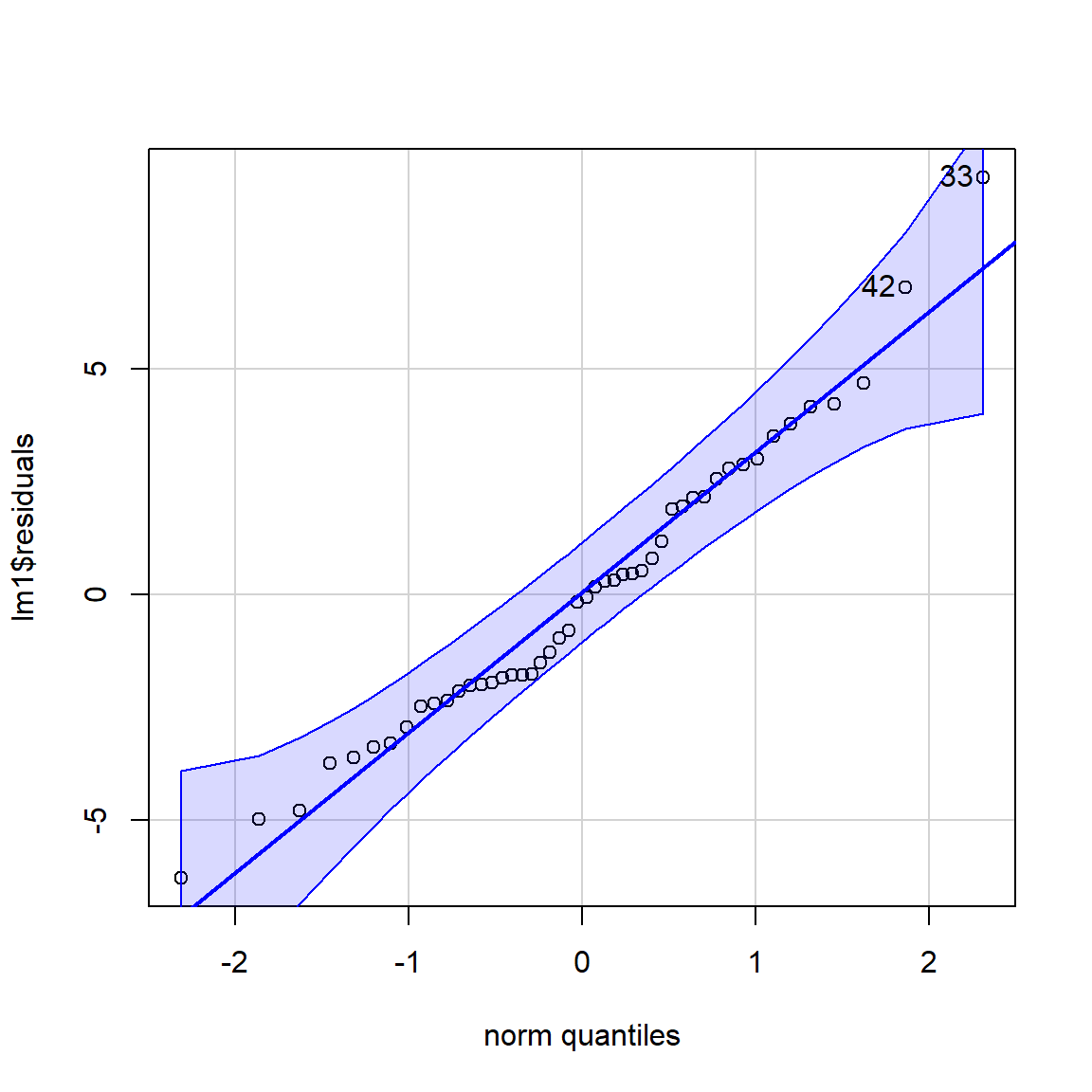
Get the normal probability plot of the model residuals.

library(car)

# get normal probability plot of the 
# regression model residuals
car::qqPlot(lm1$residuals)

33 42 
24 32 

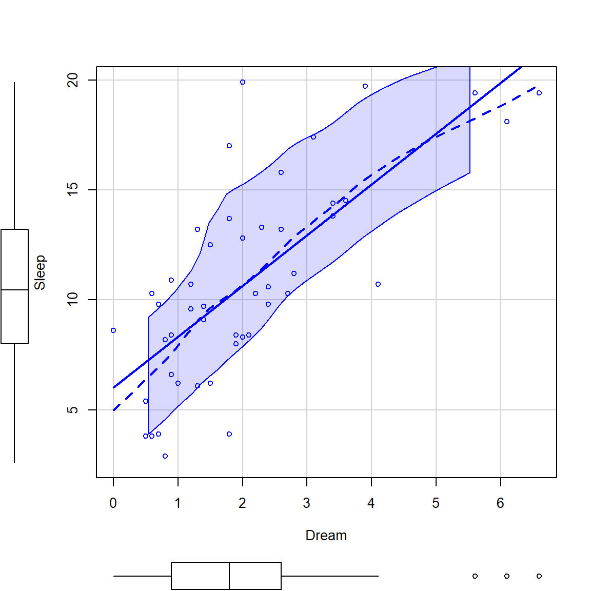
Overlay a best fit line on the scatterplot of the original data for the model - include 95% confidence intervals for the best fit line.

# scatterplot of fitted model
# using the car package, add the smooth option
car::scatterplot(Sleep ~ Dream, data = sleep, 
                 smooth=TRUE)

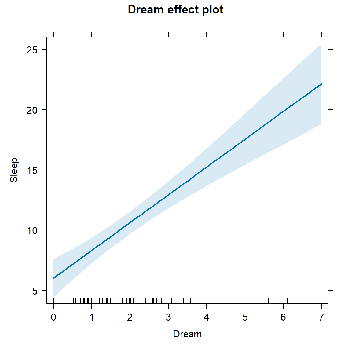
Get an “effects” plot - for this model you only get one plot showing the slope of the line between Dream and Sleep:

One more - the olsrr package

The olsrr package provides a helpful set of tolls for working with OLS (ordinary least squares) regression models. Unfortunately, this set of package functions do NOT work with glm (generalized linear models) like logistic regression.

Get detailed regression output including the standardized regression coefficients which are effect sizes, where std.beta = 0.1 is “small”, 0.3 is “moderate” and 0.5 is “large”.

# load olsrr package
library(olsrr)

# get detailed regression output
# including standardized coefficients
ols_regress(lm1)
                         Model Summary                          
---------------------------------------------------------------
R                       0.727       RMSE                 3.112 
R-Squared               0.529       MSE                  9.682 
Adj. R-Squared          0.518       Coef. Var           29.705 
Pred R-Squared          0.494       AIC                251.190 
MAE                     2.507       SBC                256.804 
---------------------------------------------------------------
 RMSE: Root Mean Square Error 
 MSE: Mean Square Error 
 MAE: Mean Absolute Error 
 AIC: Akaike Information Criteria 
 SBC: Schwarz Bayesian Criteria 

                               ANOVA                                
-------------------------------------------------------------------
               Sum of                                              
              Squares        DF    Mean Square      F         Sig. 
-------------------------------------------------------------------
Regression    521.233         1        521.233    51.593    0.0000 
Residual      464.727        46         10.103                     
Total         985.960        47                                    
-------------------------------------------------------------------

                                Parameter Estimates                                  
------------------------------------------------------------------------------------
      model     Beta    Std. Error    Std. Beta      t       Sig     lower    upper 
------------------------------------------------------------------------------------
(Intercept)    6.027         0.796                 7.572    0.000    4.425    7.630 
      Dream    2.305         0.321        0.727    7.183    0.000    1.659    2.951 
------------------------------------------------------------------------------------

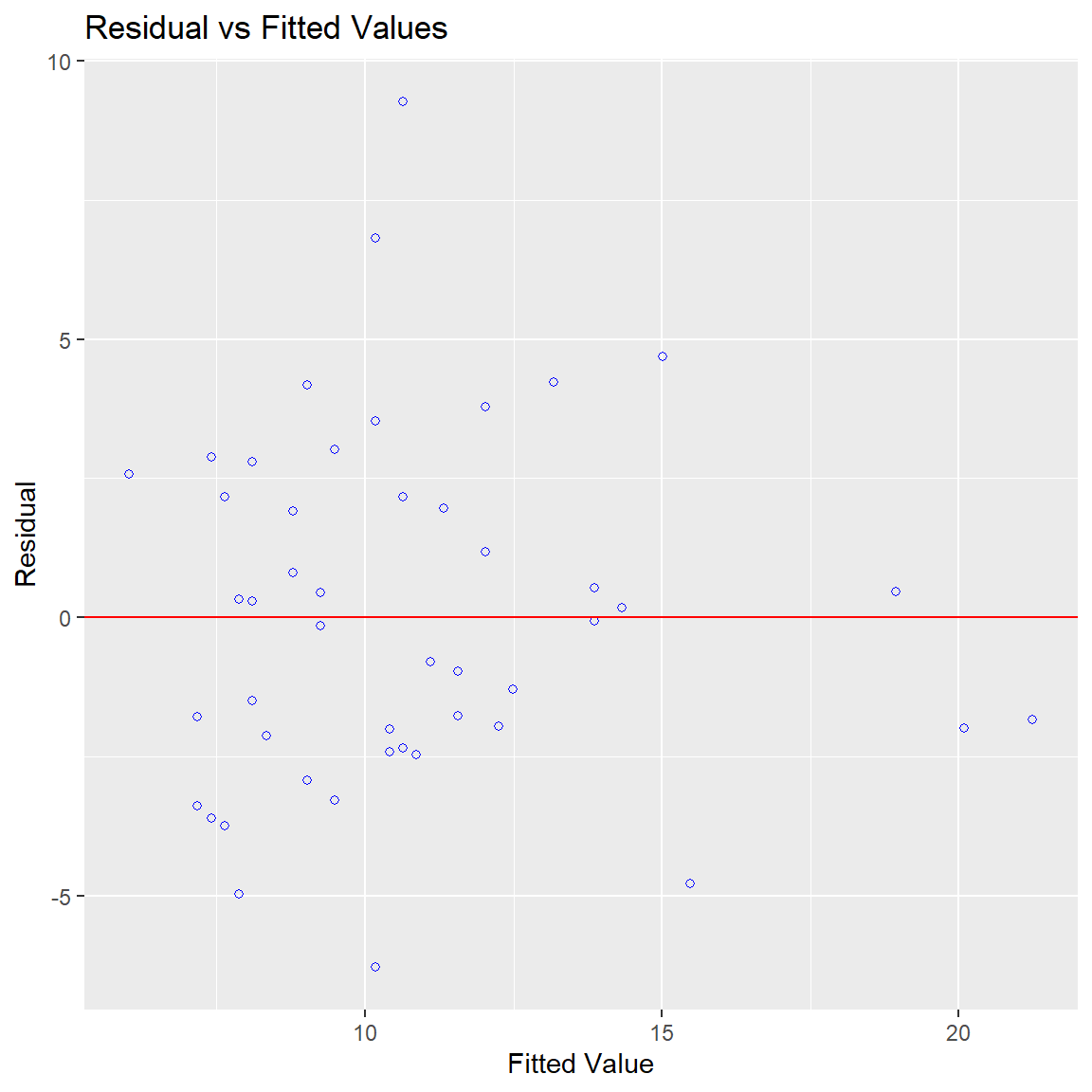
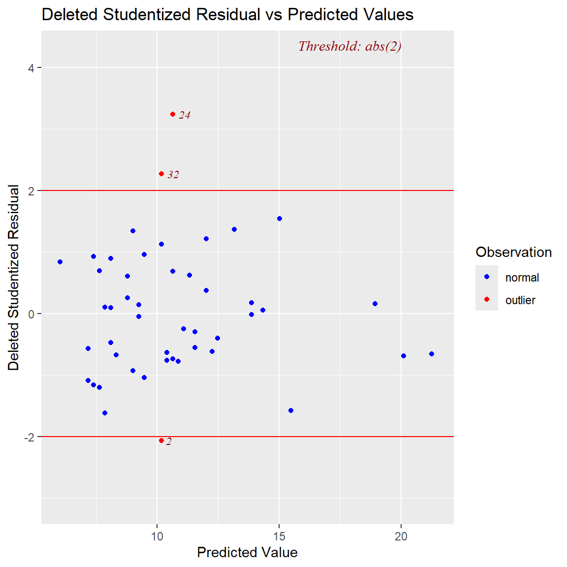
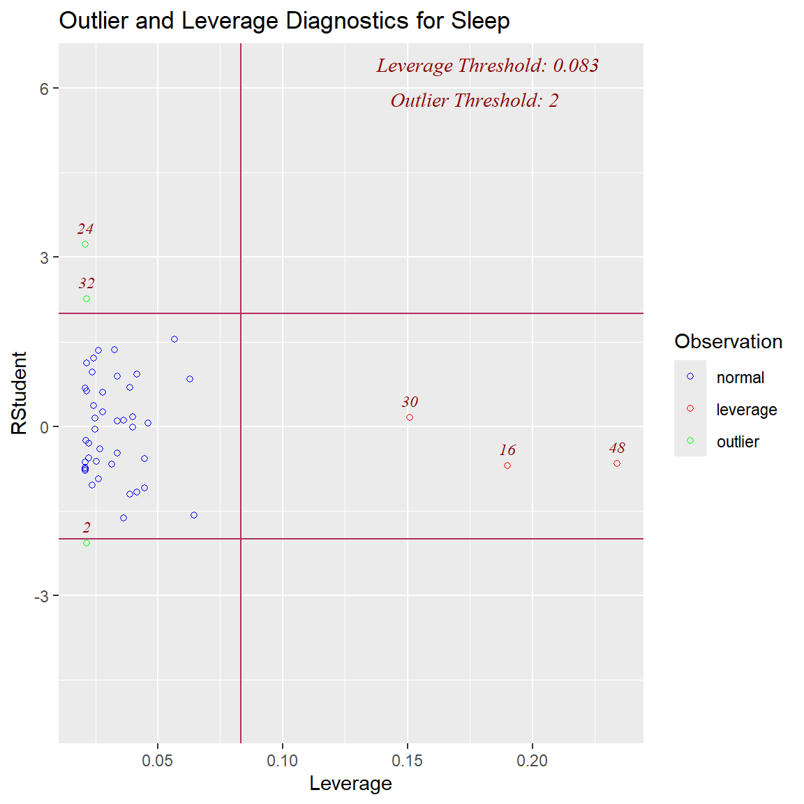
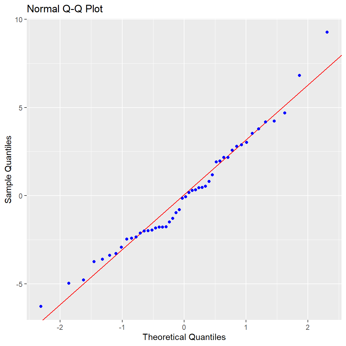
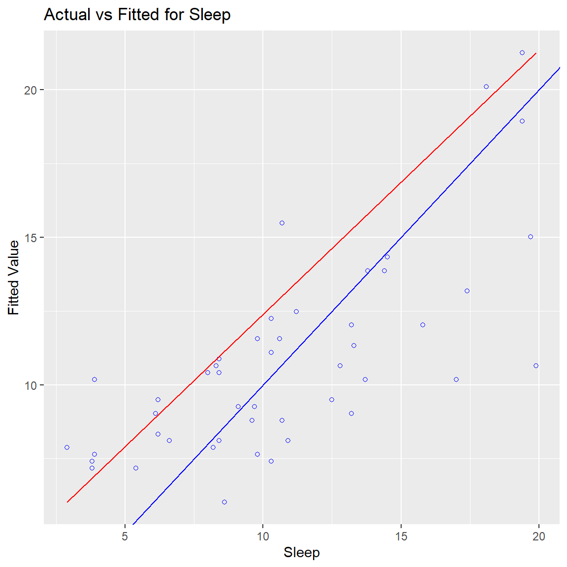
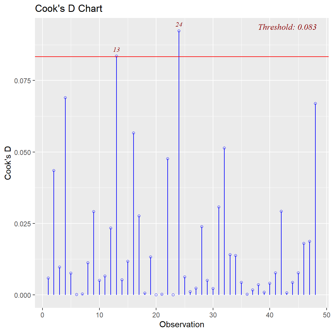
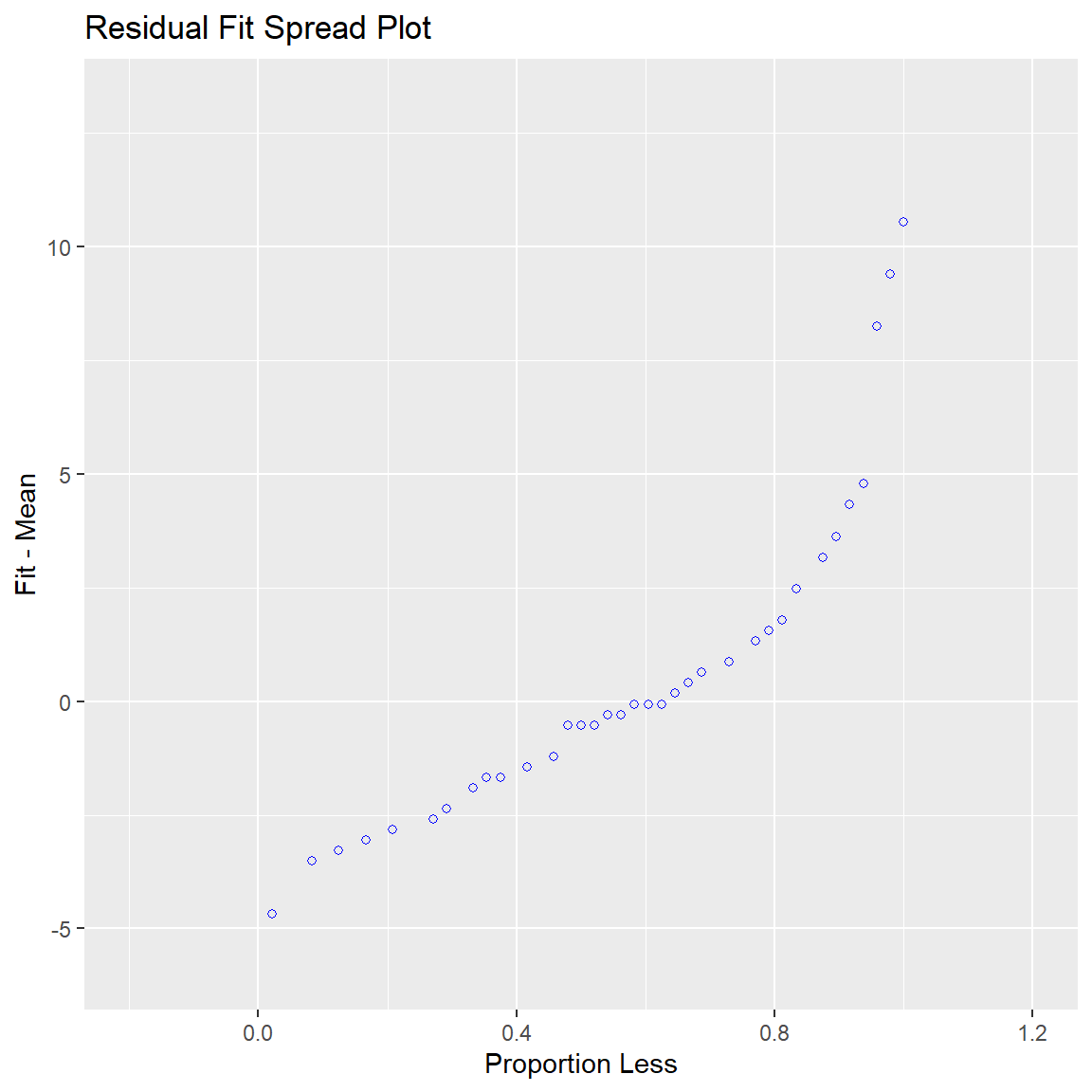
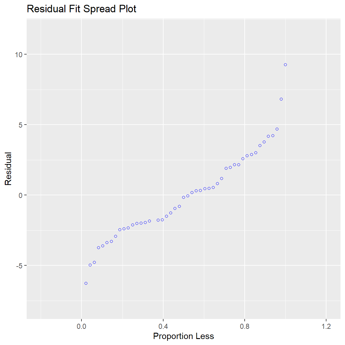
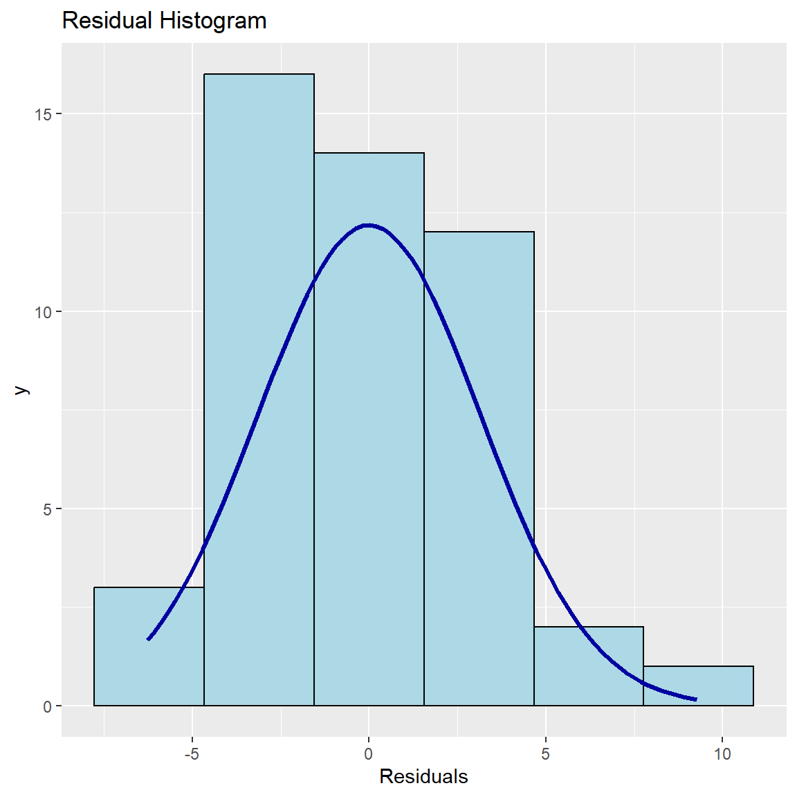
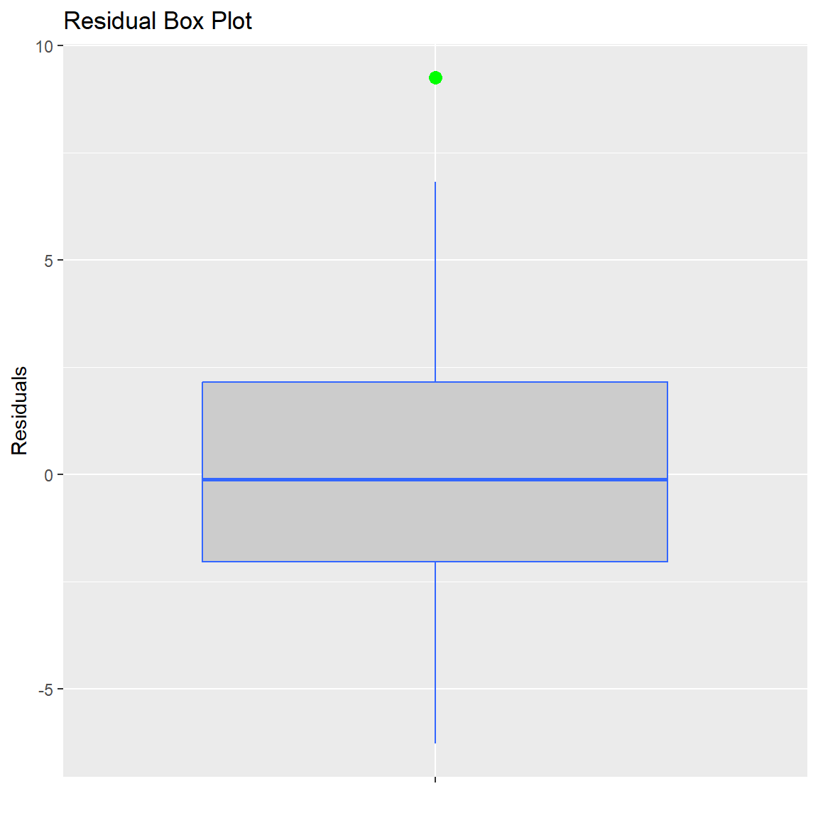
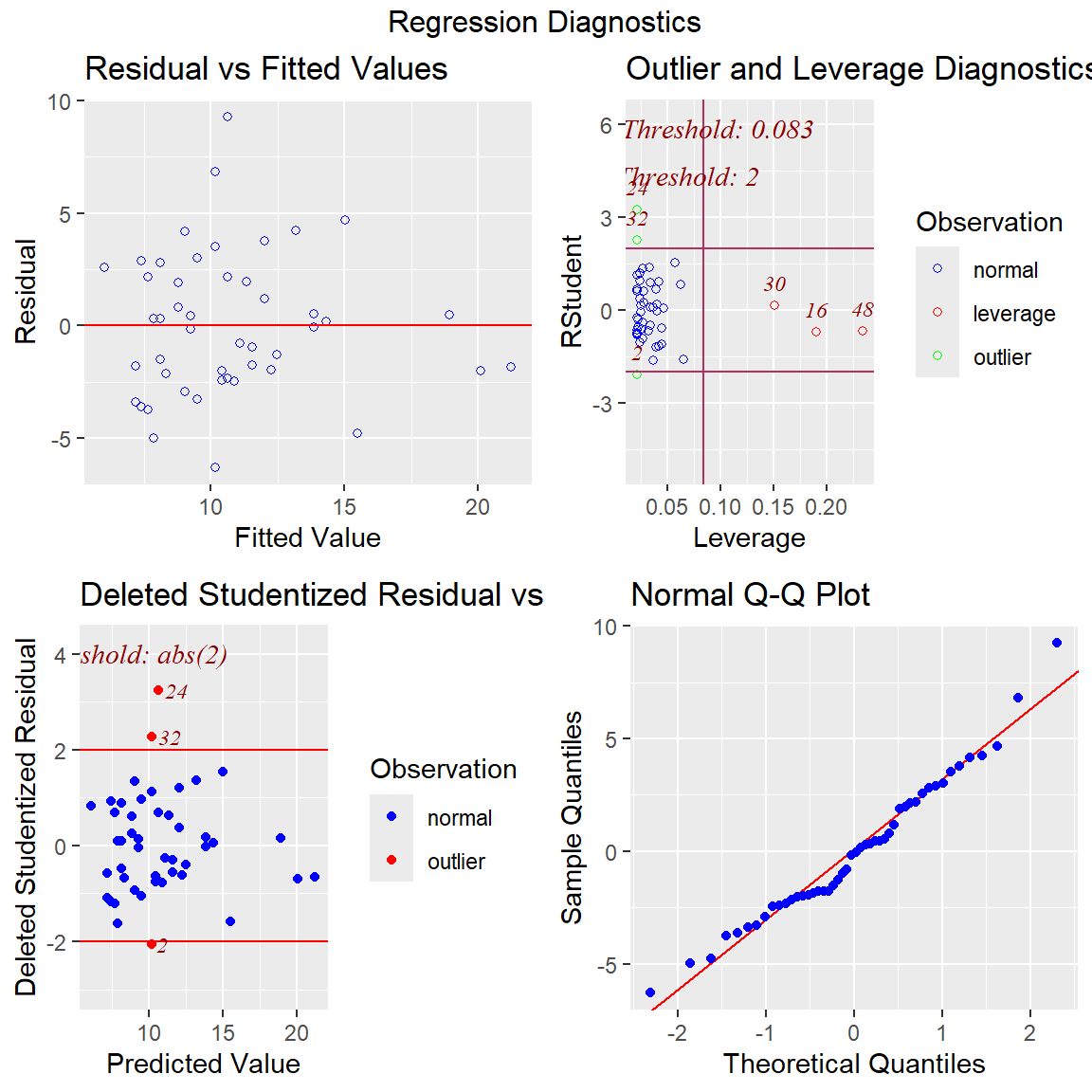
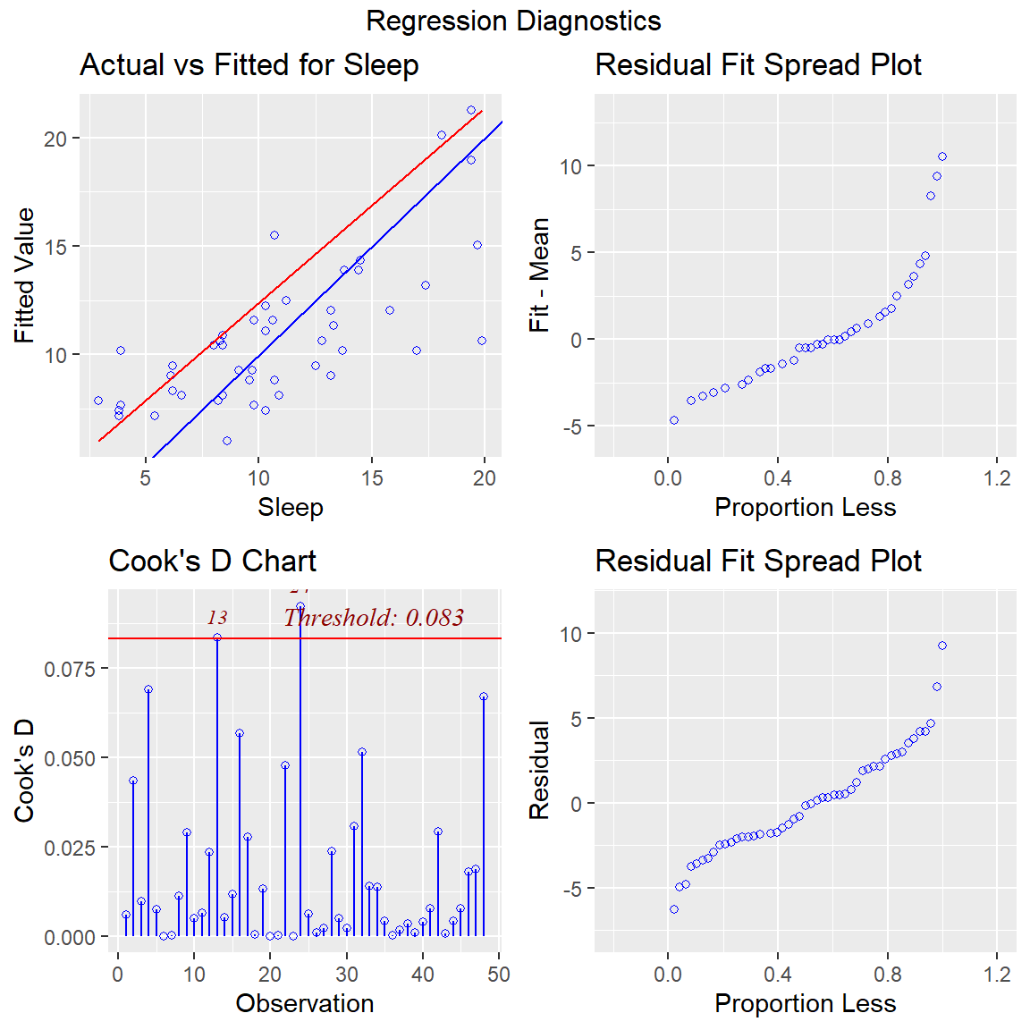
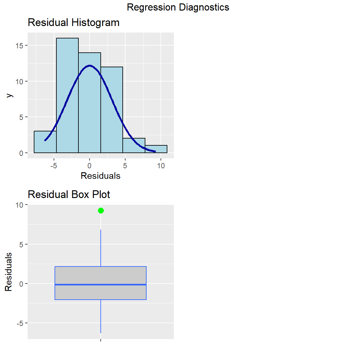
Get diagnostic plots.

# diagnostic plots
# check for new output windows
ols_plot_diagnostics(lm1)

Get a normality test for the residuals.

# normality tests for residuals
ols_test_normality(lm1)
-----------------------------------------------
       Test             Statistic       pvalue  
-----------------------------------------------
Shapiro-Wilk              0.9736         0.3468 
Kolmogorov-Smirnov        0.108          0.6307 
Cramer-von Mises          3.1824         0.0000 
Anderson-Darling          0.4289         0.2980 
-----------------------------------------------

2. Develop logistic regression models and explore results.

Similar to what we did above, we can use glm() instead of lm() to perform a logistic regression. glm() is the generalized linear modeling function in base R. The “generalized” part of this is due to this function handling different “families” of output distributions. The “gaussian” family is the default for continuous variables with a normal distribution (the assumption for OLS). The family for logistic regression is the “binomial” since we are predicting the probability of someone being in group 1 or group 2 for the 2 possible outcomes in a logistic regression. And there are more families that can be fit including “poisson” which works for count-based variables (like number of children, miscarriages, etc).

This function can actually do a simple linear regression by leaving the default setting for family = "gaussian". Learn more by running help(glm, package = "stats").

Let’s keep working with the sleep dataset, but first let’s split the Dream variable into values <= 2 and those > 2. Note: The median for Dream was 1.8, so this should split data approximately 50/50.

This time we will treat “Dream > 2” as the positive (or target) outcome for our logistic regression model. And then we will see how “Dream > 2” is predicted by amount of Sleep and Danger scores.

Simple glm() output

# create outcome variable
sleep$dream_gt2 <- as.numeric(sleep$Dream > 2)
  
# fit the logistic regression model
glm1 <- glm(dream_gt2 ~ Sleep + Danger,
            data = sleep,
            family = "binomial")

# look at basic output
glm1

Call:  glm(formula = dream_gt2 ~ Sleep + Danger, family = "binomial", 
    data = sleep)

Coefficients:
(Intercept)        Sleep       Danger  
    -1.5953       0.2677      -0.8381  

Degrees of Freedom: 47 Total (i.e. Null);  45 Residual
  (14 observations deleted due to missingness)
Null Deviance:      63.51 
Residual Deviance: 41.79    AIC: 47.79
WARNING: Exponentiate Raw Coefficients

The default output from glm() only provides for the RAW logistic regression coefficients. To get the odds ratios, we must first exponentiate these coefficients.

Get the odds ratios by exponentiating the coefficients.

exp(coef(glm1))
(Intercept)       Sleep      Danger 
  0.2028428   1.3069544   0.4325214 

Get detailed glm() regression output.

sglm1 <- summary(glm1)
sglm1

Call:
glm(formula = dream_gt2 ~ Sleep + Danger, family = "binomial", 
    data = sleep)

Coefficients:
            Estimate Std. Error z value Pr(>|z|)  
(Intercept)  -1.5953     1.5922  -1.002   0.3164  
Sleep         0.2677     0.1151   2.325   0.0201 *
Danger       -0.8381     0.3888  -2.156   0.0311 *
---
Signif. codes:  0 '***' 0.001 '**' 0.01 '*' 0.05 '.' 0.1 ' ' 1

(Dispersion parameter for binomial family taken to be 1)

    Null deviance: 63.510  on 47  degrees of freedom
Residual deviance: 41.795  on 45  degrees of freedom
  (14 observations deleted due to missingness)
AIC: 47.795

Number of Fisher Scoring iterations: 5

Use gtsummary::tbl_regression()

Get a nicer table and set exponentiate = TRUE.

tbl_regression(glm1, exponentiate = TRUE)
Characteristic OR1 95% CI1 p-value
Sleep 1.31 1.07, 1.70 0.020
Danger 0.43 0.18, 0.87 0.031
1 OR = Odds Ratio, CI = Confidence Interval

Interpret Odds Ratios as Effect Sizes

Interpreting odds ratios as effect sizes is a little tricky. However, this website on Computation of Effect Sizes is really helpful - see items 14 and 16. By playing with this simple conversion tool to convert between effect sizes, we can see that:

  • large effect sizes d=0.8, r=0.5, odds ratio =~ 4.27-8.12
  • moderate effect sizes d=0.5, r=0.3, odds ratio =~ 2.48-3.13
  • small effect sizes d=0.2, r=0.1, odds ratio =~ 1.44

where Cohen’s d is used for t-tests; r is used for correlations (and are the same for standardized regression coefficient “betas”); and odds ratios are from logistic regression.

AUC and ROC curve plot

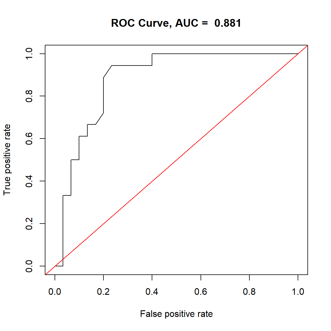
The area under the curve (AUC) or “C-statistic” is often reported instead of R2 for logistic regression models. The code below will compute the AUC for this model and make the receiver operating characteristic curve (ROC) plot.

Ideally you want AUC as close to 1 as possible:

  • AUC > 0.9 is great
  • AUC > 0.8 is good
  • AUC > 0.7 is ok
  • AUC < 0.7 is not very good
  • AUC around 0.5 is no better than flipping a fair coin which is a useless model

As you can see below, the AUC for this model was 0.881 which is very good.

# NOTE: We need only the COMPLETE data
# for the 3 variables we used in this model
library(dplyr)
s1 <- sleep %>%
  select(Sleep, Danger, dream_gt2) %>%
  filter(complete.cases(.))

# compute AUC and get ROC curve
library(ROCR)
p <- predict(glm1, newdata=s1, 
             type="response")
pr <- prediction(p, as.numeric(s1$dream_gt2))
prf <- performance(pr, measure = "tpr", x.measure = "fpr")

# compute AUC, area under the curve
# also called the C-statistic
auc <- performance(pr, measure = "auc")
auc <- auc@y.values[[1]]

# also - add title to plot with AUC in title
plot(prf,
     main = paste("ROC Curve, AUC = ", round(auc, 3)))
abline(0, 1, col="red")


3. Perform t-tests explore results.

T-tests

Given the split we did above looking at animals with Dream scores above and below 2, let’s run a t-test for the Sleep variable.

# run t-test, save results
# default is an unequal variance "unpooled" t.test
tt1 <- t.test(Sleep ~ dream_gt2, 
              data = sleep)
tt1

    Welch Two Sample t-test

data:  Sleep by dream_gt2
t = -4.5307, df = 38.191, p-value = 5.633e-05
alternative hypothesis: true difference in means between group 0 and group 1 is not equal to 0
95 percent confidence interval:
 -7.420174 -2.837604
sample estimates:
mean in group 0 mean in group 1 
       8.776667       13.905556 
# get the equal variance "pooled" t.test
tt2 <- t.test(Sleep ~ dream_gt2, 
              data = sleep,
              var.equal = TRUE)
tt2

    Two Sample t-test

data:  Sleep by dream_gt2
t = -4.4417, df = 46, p-value = 5.566e-05
alternative hypothesis: true difference in means between group 0 and group 1 is not equal to 0
95 percent confidence interval:
 -7.453219 -2.804558
sample estimates:
mean in group 0 mean in group 1 
       8.776667       13.905556 

We can test the assumption of equal variance in a couple of ways. One simple way is to look at the standard deviations of each group and see if the ratio is larger than 2.

sd0 <- sleep %>%
  filter(dream_gt2 == 0) %>%
  select(Sleep) %>%
  unlist() %>%
  sd(na.rm = TRUE)
sd1 <- sleep %>%
  filter(dream_gt2 == 1) %>%
  select(Sleep) %>%
  unlist() %>%
  sd(na.rm = TRUE)
sd0
[1] 3.980615
sd1
[1] 3.682306

These standard deviations are similar, so a pooled t-test should be fine.

You can also run a formal test of equal variance, using bartlett.test(). However, this test and others like this are sensitive to small deviations from normality, so I often check the standard deviations and will run both the pooled and unpooled tests and see if I get the same conclusion either way.

As you can see, the p-value below is not significant, so we can not reject the null hypothesis assumption of equal variance - the pooled t-test is fine.

bartlett.test(Sleep ~ dream_gt2, 
              data = sleep)

    Bartlett test of homogeneity of variances

data:  Sleep by dream_gt2
Bartlett's K-squared = 0.12522, df = 1, p-value = 0.7234

Compute effect size for t-test

Use the effectsize package which is part of the easystats suite of packages.

The effect size computed is rather large, d=1.32.

library(effectsize)
options(es.use_symbols = TRUE)

cohens_d(Sleep ~ dream_gt2, 
         data = sleep,
         na.action = na.omit)
Cohen's d |         95% CI
--------------------------
-1.32     | [-1.96, -0.67]

- Estimated using pooled SD.

Get a simple summary table

As you see below, the difference in Sleep scores between the 2 dream groups is approximately 13.9-8.8 = 5.1 and the approximate average SD =~ 3.9, so the ratio of the mean differences to “pooled” SD =~ 5.1/3.85 =~ 1.33 which is close to the Cohen’s d we computed above.

I also added some custom statistical tests to the table.

# create factor variable with labels
sleep$dream_gt2.f <- factor(
  sleep$dream_gt2, 
  levels = c(0, 1),
  labels = c("Dream <= 2",
             "Dream > 2")
)

tbl_summary(
  sleep,
  by = dream_gt2.f,
  include = c(Sleep, Danger),
  type = all_continuous() ~ "continuous2",
  statistic = all_continuous() ~ c("{N_nonmiss}", "{mean} ({sd})")
) %>%
  add_p(test = list(Sleep ~ "t.test", Danger ~ "wilcox.test"), 
        test.args = list(Sleep ~ list(var.equal = TRUE))
        ) 
Characteristic Dream <= 2
N = 321
Dream > 2
N = 181
p-value2
Sleep

<0.001
    N Non-missing 30 18
    Mean (SD) 8.8 (4.0) 13.9 (3.7)
    Unknown 2 0
Danger

<0.001
    1 5 (16%) 9 (50%)
    2 6 (19%) 6 (33%)
    3 5 (16%) 3 (17%)
    4 9 (28%) 0 (0%)
    5 7 (22%) 0 (0%)
1 n (%)
2 Two Sample t-test; Wilcoxon rank sum test

4. Modeling with Complex Survey Weights

See PRAMS Module


R Code For This Module

References

Ben-Shachar, Mattan S., Daniel Lüdecke, and Dominique Makowski. 2020. effectsize: Estimation of Effect Size Indices and Standardized Parameters.” Journal of Open Source Software 5 (56): 2815. https://doi.org/10.21105/joss.02815.
Ben-Shachar, Mattan S., Dominique Makowski, Daniel Lüdecke, Indrajeet Patil, Brenton M. Wiernik, Rémi Thériault, and Philip Waggoner. 2025. Effectsize: Indices of Effect Size. https://easystats.github.io/effectsize/.
Fox, John. 2003. “Effect Displays in R for Generalised Linear Models.” Journal of Statistical Software 8 (15): 1–27. https://doi.org/10.18637/jss.v008.i15.
Fox, John, and Jangman Hong. 2009. “Effect Displays in R for Multinomial and Proportional-Odds Logit Models: Extensions to the effects Package.” Journal of Statistical Software 32 (1): 1–24. https://doi.org/10.18637/jss.v032.i01.
Fox, John, and Sanford Weisberg. 2018. “Visualizing Fit and Lack of Fit in Complex Regression Models with Predictor Effect Plots and Partial Residuals.” Journal of Statistical Software 87 (9): 1–27. https://doi.org/10.18637/jss.v087.i09.
———. 2019a. An R Companion to Applied Regression. Third. Thousand Oaks CA: Sage. https://www.john-fox.ca/Companion/.
———. 2019b. An r Companion to Applied Regression. 3rd ed. Thousand Oaks CA: Sage. https://socialsciences.mcmaster.ca/jfox/Books/Companion/index.html.
Fox, John, Sanford Weisberg, and Brad Price. 2022. carData: Companion to Applied Regression Data Sets. https://r-forge.r-project.org/projects/car/.
———. 2024. Car: Companion to Applied Regression. https://r-forge.r-project.org/projects/car/.
Fox, John, Sanford Weisberg, Brad Price, Michael Friendly, and Jangman Hong. 2022. Effects: Effect Displays for Linear, Generalized Linear, and Other Models. https://www.r-project.org.
Hebbali, Aravind. 2024. Olsrr: Tools for Building OLS Regression Models. https://olsrr.rsquaredacademy.com/.
Iannone, Richard, Joe Cheng, Barret Schloerke, Ellis Hughes, Alexandra Lauer, JooYoung Seo, Ken Brevoort, and Olivier Roy. 2024. Gt: Easily Create Presentation-Ready Display Tables. https://gt.rstudio.com.
Ihaka, Ross, Paul Murrell, Kurt Hornik, Jason C. Fisher, Reto Stauffer, Claus O. Wilke, Claire D. McWhite, and Achim Zeileis. 2023. Colorspace: A Toolbox for Manipulating and Assessing Colors and Palettes. https://colorspace.R-Forge.R-project.org/.
Kowarik, Alexander, and Matthias Templ. 2016. “Imputation with the R Package VIM.” Journal of Statistical Software 74 (7): 1–16. https://doi.org/10.18637/jss.v074.i07.
Lüdecke, Daniel, Mattan S. Ben-Shachar, Indrajeet Patil, and Dominique Makowski. 2020. “Extracting, Computing and Exploring the Parameters of Statistical Models Using R.” Journal of Open Source Software 5 (53): 2445. https://doi.org/10.21105/joss.02445.
Lüdecke, Daniel, Mattan S. Ben-Shachar, Indrajeet Patil, Philip Waggoner, and Dominique Makowski. 2021. performance: An R Package for Assessment, Comparison and Testing of Statistical Models.” Journal of Open Source Software 6 (60): 3139. https://doi.org/10.21105/joss.03139.
Lüdecke, Daniel, Mattan S. Ben-Shachar, Indrajeet Patil, Brenton M. Wiernik, Etienne Bacher, Rémi Thériault, and Dominique Makowski. 2022. “Easystats: Framework for Easy Statistical Modeling, Visualization, and Reporting.” CRAN. https://doi.org/10.32614/CRAN.package.easystats.
Lüdecke, Daniel, Dominique Makowski, Mattan S. Ben-Shachar, Indrajeet Patil, Søren Højsgaard, and Brenton M. Wiernik. 2025. Parameters: Processing of Model Parameters. https://easystats.github.io/parameters/.
Lüdecke, Daniel, Dominique Makowski, Mattan S. Ben-Shachar, Indrajeet Patil, Philip Waggoner, Brenton M. Wiernik, and Rémi Thériault. 2025. Performance: Assessment of Regression Models Performance. https://easystats.github.io/performance/.
Lüdecke, Daniel, Dominique Makowski, Mattan S. Ben-Shachar, Indrajeet Patil, Brenton M. Wiernik, Etienne Bacher, and Rémi Thériault. 2025. Easystats: Framework for Easy Statistical Modeling, Visualization, and Reporting. https://easystats.github.io/easystats/.
Lüdecke, Daniel, Dominique Makowski, Indrajeet Patil, Mattan S. Ben-Shachar, Brenton M. Wiernik, and Philip Waggoner. 2025. See: Model Visualisation Toolbox for Easystats and Ggplot2. https://easystats.github.io/see/.
Lüdecke, Daniel, Dominique Makowski, Indrajeet Patil, Philip Waggoner, Mattan S. Ben-Shachar, Brenton M. Wiernik, Vincent Arel-Bundock, and Etienne Bacher. 2025. Insight: Easy Access to Model Information for Various Model Objects. https://easystats.github.io/insight/.
Lüdecke, Daniel, Indrajeet Patil, Mattan S. Ben-Shachar, Brenton M. Wiernik, Philip Waggoner, and Dominique Makowski. 2021. see: An R Package for Visualizing Statistical Models.” Journal of Open Source Software 6 (64): 3393. https://doi.org/10.21105/joss.03393.
Lüdecke, Daniel, Philip Waggoner, and Dominique Makowski. 2019. insight: A Unified Interface to Access Information from Model Objects in R.” Journal of Open Source Software 4 (38): 1412. https://doi.org/10.21105/joss.01412.
Makowski, Dominique, Mattan S. Ben-Shachar, and Daniel Lüdecke. 2019. “bayestestR: Describing Effects and Their Uncertainty, Existence and Significance Within the Bayesian Framework.” Journal of Open Source Software 4 (40): 1541. https://doi.org/10.21105/joss.01541.
Makowski, Dominique, Mattan S. Ben-Shachar, Indrajeet Patil, and Daniel Lüdecke. 2020. “Methods and Algorithms for Correlation Analysis in R.” Journal of Open Source Software 5 (51): 2306. https://doi.org/10.21105/joss.02306.
Makowski, Dominique, Mattan S. Ben-Shachar, Brenton M. Wiernik, Indrajeet Patil, Rémi Thériault, and Daniel Lüdecke. 2025. modelbased: An R Package to Make the Most Out of Your Statistical Models Through Marginal Means, Marginal Effects, and Model Predictions.” Journal of Open Source Software 10 (109): 7969. https://doi.org/10.21105/joss.07969.
Makowski, Dominique, Daniel Lüdecke, Mattan S. Ben-Shachar, Indrajeet Patil, and Rémi Thériault. 2025. Modelbased: Estimation of Model-Based Predictions, Contrasts and Means. https://easystats.github.io/modelbased/.
Makowski, Dominique, Daniel Lüdecke, Mattan S. Ben-Shachar, Indrajeet Patil, Micah K. Wilson, and Brenton M. Wiernik. 2025. bayestestR: Understand and Describe Bayesian Models and Posterior Distributions. https://easystats.github.io/bayestestR/.
Makowski, Dominique, Daniel Lüdecke, Indrajeet Patil, Rémi Thériault, Mattan S. Ben-Shachar, and Brenton M. Wiernik. 2023. “Automated Results Reporting as a Practical Tool to Improve Reproducibility and Methodological Best Practices Adoption.” CRAN. https://easystats.github.io/report/.
———. 2025. Report: Automated Reporting of Results and Statistical Models. https://easystats.github.io/report/.
Makowski, Dominique, Brenton M. Wiernik, Indrajeet Patil, Daniel Lüdecke, and Mattan S. Ben-Shachar. 2022. correlation: Methods for Correlation Analysis.” https://CRAN.R-project.org/package=correlation.
Makowski, Dominique, Brenton M. Wiernik, Indrajeet Patil, Daniel Lüdecke, Mattan S. Ben-Shachar, and Rémi Thériault. 2025. Correlation: Methods for Correlation Analysis. https://easystats.github.io/correlation/.
Patil, Indrajeet, Etienne Bacher, Dominique Makowski, Daniel Lüdecke, Mattan S. Ben-Shachar, and Brenton M. Wiernik. 2025. Datawizard: Easy Data Wrangling and Statistical Transformations. https://easystats.github.io/datawizard/.
Patil, Indrajeet, Dominique Makowski, Mattan S. Ben-Shachar, Brenton M. Wiernik, Etienne Bacher, and Daniel Lüdecke. 2022. datawizard: An R Package for Easy Data Preparation and Statistical Transformations.” Journal of Open Source Software 7 (78): 4684. https://doi.org/10.21105/joss.04684.
R Core Team. 2025. R: A Language and Environment for Statistical Computing. Vienna, Austria: R Foundation for Statistical Computing. https://www.R-project.org/.
Robinson, David, Alex Hayes, and Simon Couch. 2025. Broom: Convert Statistical Objects into Tidy Tibbles. https://broom.tidymodels.org/.
Sing, Tobias, Oliver Sander, Niko Beerenwinkel, and Thomas Lengauer. 2020. ROCR: Visualizing the Performance of Scoring Classifiers. http://ipa-tys.github.io/ROCR/.
Sing, T., O. Sander, N. Beerenwinkel, and T. Lengauer. 2005. “ROCR: Visualizing Classifier Performance in r.” Bioinformatics 21 (20): 7881. http://rocr.bioinf.mpi-sb.mpg.de.
Sjoberg, Daniel D., Joseph Larmarange, Michael Curry, Jessica Lavery, Karissa Whiting, and Emily C. Zabor. 2024. Gtsummary: Presentation-Ready Data Summary and Analytic Result Tables. https://github.com/ddsjoberg/gtsummary.
Sjoberg, Daniel D., Karissa Whiting, Michael Curry, Jessica A. Lavery, and Joseph Larmarange. 2021. “Reproducible Summary Tables with the Gtsummary Package.” The R Journal 13: 570–80. https://doi.org/10.32614/RJ-2021-053.
Stauffer, Reto, Georg J. Mayr, Markus Dabernig, and Achim Zeileis. 2009. “Somewhere over the Rainbow: How to Make Effective Use of Colors in Meteorological Visualizations.” Bulletin of the American Meteorological Society 96 (2): 203–16. https://doi.org/10.1175/BAMS-D-13-00155.1.
Templ, Matthias, Alexander Kowarik, Andreas Alfons, Gregor de Cillia, and Wolfgang Rannetbauer. 2022. VIM: Visualization and Imputation of Missing Values. https://github.com/statistikat/VIM.
Wickham, Hadley, Romain François, Lionel Henry, Kirill Müller, and Davis Vaughan. 2023. Dplyr: A Grammar of Data Manipulation. https://dplyr.tidyverse.org.
Zeileis, Achim, Jason C. Fisher, Kurt Hornik, Ross Ihaka, Claire D. McWhite, Paul Murrell, Reto Stauffer, and Claus O. Wilke. 2020. colorspace: A Toolbox for Manipulating and Assessing Colors and Palettes.” Journal of Statistical Software 96 (1): 1–49. https://doi.org/10.18637/jss.v096.i01.
Zeileis, Achim, Kurt Hornik, and Paul Murrell. 2009. “Escaping RGBland: Selecting Colors for Statistical Graphics.” Computational Statistics & Data Analysis 53 (9): 3259–70. https://doi.org/10.1016/j.csda.2008.11.033.

Other Helpful Resources

Other Helpful Resources